Category: Excel formulas and functions

Excel formulas and functions are part of the essentials that everyone should learn about Microsoft Excel. Excel formulas and functions They serve to get the most out of the tools which offers the most used spreadsheet in the world. 

Imagine for a moment that Excel is a vast ocean. There, each formula and function is a unique species. Some are simple and easy to understand, like the friendly dolphins that represent our basic ADDITION and SUBTRACTION formulas. Others are more complex and mysterious, like the blue whales that symbolize advanced functions such as VLOOKUP or SUMIF.

But do not worry, You don't need to be a marine biologist to explore this ocean. Like a compass, this article will guide you through the depths of Excel. We will reveal the secrets of its inhabitants and We'll show you how they can help you navigate your own seas of data.

So put on your wetsuit, adjust your goggles, and get ready to immerse yourself in the fascinating world of Excel formulas and functions. Let's explore together!

First: What is an Excel formula?

Excel formulas They are mathematical operations that we enter in a cell. Each of these expressions will give us a result, which will be shown in the cell where we write the formula.  

Imagine that Excel is like a big calculator. Instead of having to do calculations in your head or on a piece of paper, you can write what you want to calculate in Excel and it will do the work for you.

A formula in Excel is like a cooking recipe. It tells you exactly what ingredients you need (the data in your cells) and how to combine them (the math) to get the result you want.

For example, if you have a list of prices in a column and you want to know how much it would cost to buy one of each item, you could use a formula to add all the prices. That formula will look like: =(A1+A2+A3). You can perform the same action if you want to perform other mathematical operations such as subtraction, division or multiplication. 

And now, what is an Excel function?

Excel functions are specific formulas that Excel already has built-in. Each function has its name and specific structure. It is also defined as a predefined formula that performs a specific calculation based on the values you provide it. Excel has a wide variety of functions you can use, each designed to perform a specific type of calculation.

For example, the SUM(A1:A3) function Add the values in cells A1 to A3. The AVERAGE(B1:B10) function calculates the average of the values in cells B1 through B10. And the VLOOKUP function can look up a value in a table and return a corresponding value from another column.

What is the difference between a formula and an Excel function?

In Excel, both formulas and functions are used to calculate and manipulate data in cells. However, there is a key difference between them:

What is a Formula?

It is an expression that performs calculations on cell values. You can use basic mathematical operators such as addition (+), subtraction (-), multiplication (*) and division (/). For example, if you have the number 5 in cell A1 and number 10 in cell A2, you can add these two numbers with the formula =(A1+A2).

What is a function?

It is a special type of predefined formula that performs a specific calculation. Excel has more than 100 built-in functions to perform a variety of calculations. For example, you can use the fSUM function to sum a range of cells, such as SUM(A1:A10), which would sum all the numbers in cells A1 to A10.

In short, all functions are formulas, but not all formulas are functions. Formulas are more general and can consist of simple mathematical operations, while functions are predefined operations that perform specific calculations.

What elements make up a formula in Excel?

A formula in Excel is made up of several elements that are essential to make calculations. Here are the key components:

• Equal sign (=): All formulas in Excel start with an equal sign. It tells Excel that what follows is a formula.
  
• Cells and cell ranges: Formulas typically refer to individual cells (such as A1) or ranges of cells (such as A1:A10) to perform calculations on the data in those cells.
  
• Operators: The operators are the symbols that indicate the type of calculation that must be performed. Basic operators include + for addition, – for subtraction, * for multiplication, and / for division.
  
• Features: Functions are predefined calculations that you can use in your formulas. For example, SUM(A1:A10) adds all the numbers in cells A1 through A10.
  
• Constants: Constants are values that do not change. For example, in the formula =A1+10, the number 10 is a constant.

Here's a simple example of what these elements look like in a formula:
Suppose you have the number 5 in cell A1 and the number 10 in cell A2. If you want to add these two numbers and subtract 3, you could use the formula =A1+A2-3. In this formula:

The equal sign (=) at the beginning tells Excel that this is a formula.
A1 and A2 are cell references. The plus (+) and minus (-) signs are operators. The number 3 is a constant.

What is the formula bar in Excel for?

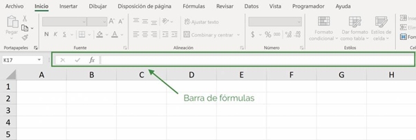
The formula bar in Excel is a tool that allows you to write and edit formulas or functions in your cells. It is located at the top of the Excel sheet, just below the ribbon.

When you select a cell, the formula bar displays the contents of that cell. If the cell contains a formula or function, you can see exactly what calculations are being performed. 

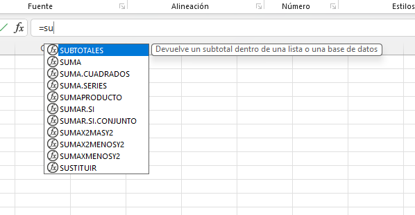
Additionally, the formula bar provides you with useful information when you are writing or editing formulas and functions. For example, if you are writing a function, Excel will show you a drop-down list with Suggestions for functions you can use. It will also give you information about the arguments each function needs.

In this bar we can see the data content or formulas that has the active cell (selected) and modify it if we want.

How to create formulas in Excel?

Inserting Excel formulas and functions helps us perform different calculations in a simple way. Excel simplifies calculations and gives us a result quickly without having to have a calculator.

How do we do it? We click on the cell where we want to insert the Excel formula, and we put an equal sign (“=”) so that Excel identifies that it is a formula.

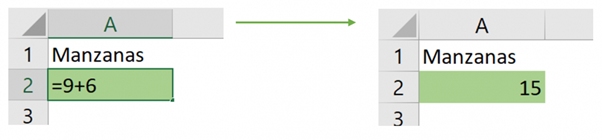
Then, we can make two types of formulas: with numbers directly, or with cell references. Let's imagine the following example, where we have to add the number of apples that are in 2 different places. In one place there are 9 apples and in the other place there are 6 apples how do we add?

1. Excel formulas only with numbers: Simply after entering the equal sign, we put 9+6, press “Enter”, and Excel automatically gives us the result we want: 15 apples in total.

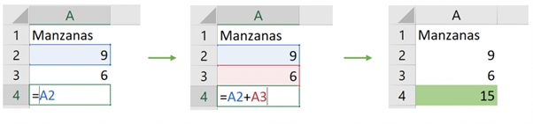
2. Excel formulas with cell references: now each number is in a different cell, and we can use its cell references to perform the operation we want.

As? We put an equal sign, we select the cell where the number 9 is (A2), then we use the plus sign (+), we select the cell where the number 6 is (A3) and finally we press “Enter”.

Thus, Excel gives us the desired result as we see in the image. Besides, Excel associates a color for each cell reference, which makes it easier for us to visualize the Excel formulas.

What is the purpose of doing this? Being based on the cells, and not the numbers, we can change the value of the cells.

What does it mean? the result will also change! In our example, if in A2 instead of putting a 9, we put a 14, the value of our result automatically changes and we are left with the value of 20 instead of 15, as we see in the image below the formula remains the same! It's still A2 + A3.

What are the types of formulas that exist in Excel? 

In Excel, there are several types of formulas that you can use, depending on what you need to calculate or the task you are performing. Here I present some types of formulas that you could find:

1. Arithmetic formulas: These are the most basic formulas and perform mathematical operations such as addition (+), subtraction (-), multiplication (*) and division (/). For example, the formula =(A1+A2) adds the values in cells A1 and A21.
2. Text formulas: These formulas allow you to manipulate text. For example, you can use the CONCATENATE (or simply &) function to join two or more texts.
3. Date and time formulas: Excel has a series of formulas that allow you to work with dates and times. For example, you can use the NOW function to get the current date and time. 
4. Logical formulas: These formulas allow you to perform logical tests that return TRUE or FALSE. For example, you can use the IF function to perform one action when a condition is met and another action if it is not met.
5. Search and reference formulas: These formulas allow you to search for data in your spreadsheet. For example, you can use the VLOOKUP function to look up a value in one column and return a value from another column. 
6. Statistics formulas: These formulas allow you to perform statistical calculations. For example, you can use the AVERAGE function to calculate the average of a range of cells.
7. Financial formulas: These formulas are useful for making financial calculations. For example, you can use the PAYMENT function to calculate a loan payment based on a constant interest rate.
8. Engineering formulas: These formulas are useful for solving engineering and design problems. 

It's time to dive into the formulas! Below you will find the most used formulas in Microsoft Excel and how to do it.

 

Basic Excel Formulas

Review the list of the most basic Excel functions and formulas below:

Formula to add

The sum formula in Excel is one of the simplest of all. You can add any type of number (positive, negative, decimal, etc.) as many times as you want. For this we use the “+” symbol. For example, to add cells C3, C4 and C5 I have to write: “=C3+C4+C5”.

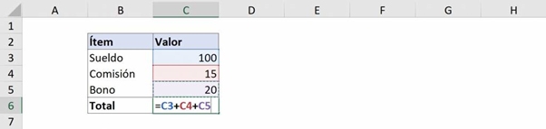
If you look, within the formula each cell we write has a different color. In this way, the selected cell is colored with that same color so that it is easy for us to see which cells we are adding.

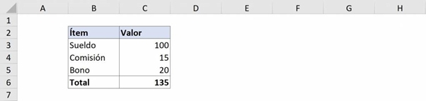
We can also use the SUM function, in which we must select all the cells that we want to add without having to write “+”.

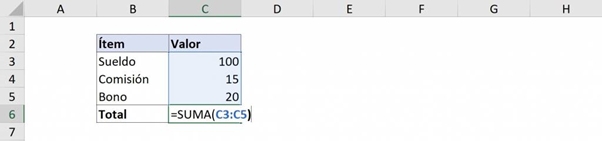
With both methods we obtain:

formula for subtraction

In the same way as to add, We use the symbol “-“ to subtract. It can also be used for all types of numbers and can be subtracted as many times as we want in a single formula. For example, to subtract C4 and C5 to C3 we would write “=C3-C4-C5”.

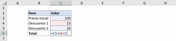
Getting:

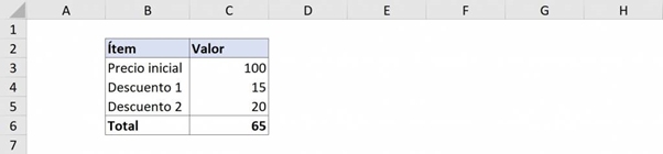
In Excel there is no SUBSTRUCTION function. However, we can use the addition function and add a negative number to it to result in a subtraction.

Formula to multiply

To do multiplications in Excel we must use an asterisk “*” to multiply two values. Like addition and subtraction, it works for all types of numbers and can be used as many times as we want in a formula.

For example, for To calculate the final price of a product we need to add VAT and incorporate a discount. For that we will combine addition and multiplication, writing: “=C3*(1+C4)*(1-C5)”

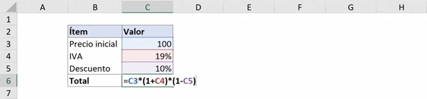
Ninja Tip: We can combine the operations addition, subtraction, multiplication and division in the same way as on a calculator: first the multiplication and division are calculated and then addition and subtraction, obeying the order of parentheses.

Formula to divide

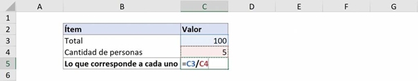
To make divisions in Excel we must use a forward slash “/” to divide two values. Like addition and subtraction, it works for all types of numbers and can be used as many times as we want in a formula.

For example, to divide a total of 100 into 5 equal parts we write “=C3/C4”.

MAX and MIN function

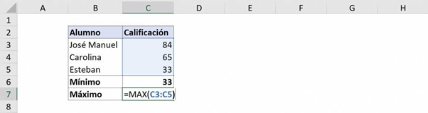
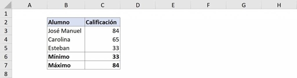
The functions MAX and MIN find the maximum and minimum of a set of numbers, respectively. For example, for a list of ratings we want to know the minimum and maximum. To obtain the minimum we write: “=MIN(C3:C5)”:

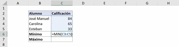
And to get the maximum we write: “=MAX(C3:C5)”:

Finally obtaining:

AVERAGE function

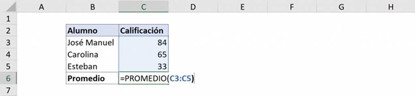
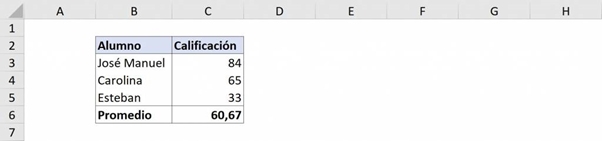
The AVERAGE function results in the average of the selected numbers. For example, to obtain the average of certain grades we write: “=AVERAGE(C3:C5)”:

Getting:

 

VLOOKUP function

The VLOOKUP function searches for elements of a table or range by row depending on a value. For example, when writing “=VLOOKUP(H2;B2:E5;2;0)” we want the first column to search for “Esteban” and return what it says in column 4 of that same row.

Thus, we obtain:

Percent formula

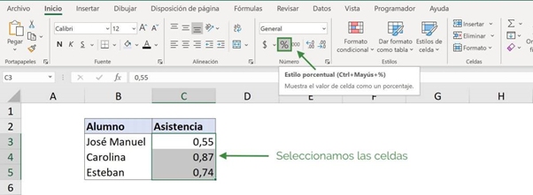
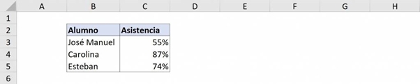
There is no formula to return numbers to percentage, but rather it is a formatting style. This can be applied by selecting the cells and searching for this format in the ribbon, as seen in the following image:

So the result is:

ROUND function

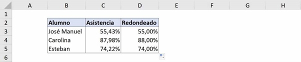
To round numbers, use the ROUND function, which has two arguments: the cell that you want to round and the number of decimal places that we want. As in the following example where we want to leave only two decimal places, we write: “ROUND(C3;2)”.

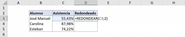
Applying it to all cells we obtain:

Advanced Excel Features

In the following list you can review the Excel formulas and functions, considered intermediate or advanced level:

Mathematical and Trigonometric Functions

ADD IF: The SUMIF function in Excel is used to sum the values in a range that meet the criteria you have specified. For example, if you want to add values greater than 5 in a range of cells, use the following formula: =SUMIF(B2:B25;”>5″)

SUM IF SET: Sums values by adding all arguments that meet multiple criteria. Unlike the SUMIF function that allows a single criterion, the SUMIF SET function allows up to 127 criteria. 

MMULT: This function returns the matrix product of two matrices. The result is a matrix with the same number of rows as matrix1 and the same number of columns as matrix. Multiply two matrices.

COUNT: Used to count the number of cells containing numbers within a range or array of numbers. For example, you can write the following formula to count the numbers in the range A1:A20: =COUNT(A1:A20). In this example, if five of the cells in the range contain numbers, the result is 5. 

COUNT IF SET: Counts the number of selected cells that meet certain conditions defined by us.

 

WHOLE: Returns the integer part of a number.

AVERAGE: The function AVERAGE in Excel returns the average (arithmetic mean) of the arguments. For example, if the range A1:A20 contains numbers, the formula =AVERAGE(A1:A20) returns the average of those numbers. 

AVERAGE IF JOINT: Calculates the average of the contents of selected cells if they meet certain conditions defined by us.

ROUND OUT: The ROUND function in Excel rounds a number to a specified number of decimal places. For example, if cell A1 contains 23.7825 and you want to round that value to two decimal places, you can use the following formula: =ROUND(A1; 2). The result of this function is 23,781.

Financial Functions

TIR function: This function calculates the internal rate of return of the cash flows represented by the numbers in the values argument. These cash flows do not have to be constant, as is the case in an annuity.

VNA function: Calculate the Net Present Value (NPV) of a set of periodic cash flows. This function allows knowing the current value of an investment and being able to compare it with the initial investment, analyzing whether it will be gained or lost.

NPER function: Returns the number of periods for an investment based on constant periodic payments and a constant interest rate.

RATE function: Returns the interest rate per period of an annuity.

VA function: Returns the Present Value (PV) of a set of periodic cash flows.

PAYMENT Function: Calculates a loan payment based on constant payments and a constant interest rate.

VF function: Returns the Future Value (FV) of a set of periodic cash flows.

PAGOPRIN function: Calculates the amortization amount of principal and interest contained in the installment of an amortizable loan with a fixed interest rate.

PAGOINT function: Calculates the amount corresponding to the interest contained in the installment of an amortizable loan with a fixed interest rate.

TIRM function: Returns the modified internal rate of return for a series of periodic cash flows. The cost of the investment and the interest obtained by reinvesting the money are considered.

Logic Functions

IF function: Make logical comparisons between a value and an expected result.

AND function: Evaluates several logical expressions and allows us to know if all of them are true.

It worked: Evaluates several logical expressions and allows us to know if any of them are true.

IF SET function: Makes logical comparisons between a value and an expected result considering various conditions.

IFERROR function: Returns a value that we specify if a formula evaluates it as an error. If there is no error, it returns the result of the formula.

YES.ND function: a value that we specify if a formula returns the error value #N/A. If there is no error, it returns the result of the formula.

Text Features

RIGHT function: It is used to extract a subtext from a text string starting with the rightmost character, taking into account the number of characters that we specify.

LEFT function: It is used to extract a subtext from a text string starting with the leftmost character, taking into account the number of characters that we specify.

CONCATENATE function: Joins two or more text strings into one.

SPACES function: Eliminates spaces from the text, except the normal space left between words.

LONG function: Calculates the number of characters inside an Excel cell.

EXTRA function: Returns a specific number of characters from a text string, starting at the position with the number of characters that we specify.

FIND function: Returns the position within a text string where it finds a character that we specify.

Date and time functions

TODAY Feature: Shows today's date. It is updated every time we open the form.

NOW Feature: Shows the current date and time. It is updated every time we open the form.

DATEIF function: Calculates the number of days, months or years between two dates.

WORKDAYS function: Calculates the number of business days (or business days) between two dates.

YEAR function: Returns the year (between 1900 and 9999) of the given date.

DATE function: Returns the sequential serial number (dd/mm/yyyy) that represents a given date.

TIME function: Returns the time (the integer value) of a time value. The time is expressed between 0 (12:00 AM) and 23 (11:00 PM).

Functions of searching and referencing

INDEX function: Returns the value contained in a cell having given the row and column number.

VLOOKUP function: Looks for a value in the first column of a table and then returns a value in the same row from a column specified by us.

XLOOKUP function: Searches one column for a search term and returns a result from the same row in another column, regardless of which side the returned column is on.

MATCH function: Searches for a given element in a range of cells and returns the relative position of that element in the range.

TRANSPOSE function: Rotates the selected data, changing rows for columns.

COUNT function: Counts the number of cells that contain numbers.

CORREL COEF function: Returns the correlation coefficient of two cell ranges.

COUNTIF function: Counts the number of cells that contain numbers under some condition that we have defined.

COUNT function: Counts the number of cells that contain any type of content (it does not differentiate numbers, texts, etc.).

Other Functions that may be useful to you 

ROW function: Returns the row number of a reference.

COLUMN function: Return the number of the column to their reference.

RANDOM function: Returns a random number between 0 and 1.

NPV function: It is the same as the VNA function.

AV CONSULT function: Is the same as VLOOKUP.

Examples of the most used Excel functions and formulas

IF function:

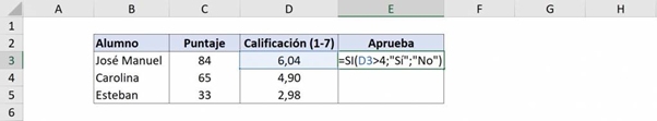
In this example we have three students who have a score and grade that is between 1 and 7. We want to create a function that tells us that you do pass the subject if the grade is greater than 4 and not if it is less than or equal to 4. Thus, we write: =IF(D3>4;”Yes”;”No”).

The first argument of this function is the condition that we want to be met, in this case it is D4>4, that is, that José Manuel's grade is greater than 4. 

Then, the next argument is the value that the function takes if the condition is met, in this case it is the word Yes, which is enclosed in quotes because it is text. 

Finally, the last argument is the value that the cell takes if the condition is not met, in this case it is the word No, which must also be enclosed in quotes.

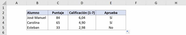
If we apply this to the entire table we obtain:

VLOOKUP function:

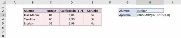
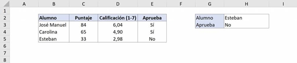
We will start from the result of the previous example and we will put ourselves in the position of wanting to know if Esteban passed the subject or not. For that we use the VLOOKUP function and we write “=VLOOKUP(H2;B2:E5;2;0)”.

The first argument of the function is the value we are looking for, in this case H2, because that is the name we are looking for. Then, the next argument is the table where the data is. Then, the next argument is the column number where the result we want is: in this case it is the fourth column that tells us whether it passed or not. Finally, the last argument is whether an exact match is needed or not.

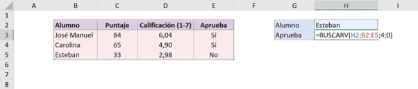
Thus, we obtain:

Formula to subtract and add in Excel

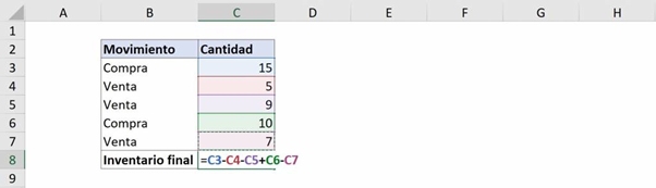
In the following example we have how many units have been bought and sold in a store and we want to know how many units are finally left. For that we will combine the addition and subtraction, writing “=C3-C4-C5+C6-C7”, so I add all the purchases and subtract the sales.

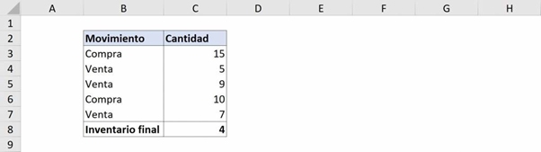
Finally, the result is 4 units in the final inventory:

Frequently asked questions about Excel formulas and functions

How to insert Formulas in Excel?

1. We click on the cell of the spreadsheet where we want to enter the formula
2. We write the equals sign (“=”) followed by the Excel formula or function that you want to use in the calculation. For example we write “=1+1”.
3. We press Enter (or Return on Mac) and we get “2” in that cell.

For more details on this you can go to this section of this article

How to copy formulas in Excel?

1. We select the cell we want to copy
2. We press Ctrl+C (or Cmd+C on Mac) to copy. We can also right click and select “Copy”.
3. We select the cell where we want to paste it.
4. We press Ctrl+V (or Cmd+V on Mac) to copy. We can also right click and select “Paste” or go to the ribbon and click “Paste”.

Tip Ninja: Clicking the arrow next to “Paste” on the ribbon opens several paste options. The most commons are:

• Formulas: Only the cell formula is pasted but not the format
• Formulas and number format: Both formula and number format (percentage format, currency format, etc.) are pasted.
• Keep source format: Both formula and number format, font, size, border and shading are pasted.
• Paste values: Only the result is pasted, without the original formula.

If we need to copy the formula to adjacent cells, we can use the “Fill Controller”.

1. We write the formula in the first cell that we want to fill:
2. We select the cell that contains the formula with which we want to fill the adjacent cells.
3. We place the cursor (or mouse) in the lower right corner so that it becomes a plus sign (“+”). This is what is known as a “filler driver.” 
4. We drag the fill handle down, up or across all the cells you want to fill. In this case we will drag to the bottom.
5. When you release, the formula is automatically inserted into the other cells:

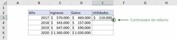
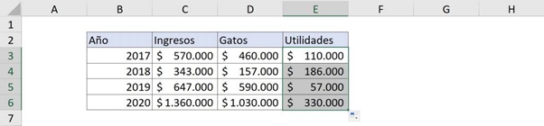
Tip Ninja: Note that the formula is pasted using relative references, i.e. the formula in cell E6 says “=C6-D6”. To learn about relative, absolute and mixed references you can see this Ninja article.

What are the 10 most used formulas in Excel?

ADDITION

COUNT

WILL COUNT

COUNT.YEAH

YEAH

VLOOKUP

HLOOKUP

ADD IF and AVERAGEIF

CONCATENATE

RANDOM