LOOKUP function in Excel: find values easily

The SEARCH function in Excel is a useful tool that allows you to search for a specific value in a range of cells. This way a corresponding value will be returned from the same place in a second range. This function can be used in two ways: vector and matrix.

Vector shape:

• search_value (mandatory): It is the value you want to find.
• comparison_vector (required): A range of cells that is made up of a single column or a single row where the search will be performed.
• result_vector (optional): The range of cells that contains the column or row of results you want to obtain.

matrix form

• search_value (mandatory): It is the value you want to find.
• Matrix (required): An array of values that contains both the search and result values.

In the next Ninja Excel article, you will know the best way to use this search function. Let's get started!

Key information

The SEARCH function allows you to search for elements in a table. The elements this function looks for must be in a given cell range (“comparison_vector”) and it will return the data of the column that you indicate in “result_vector”. You can also use the SEARCH function to find values in an array. If the searched value is not found in the table, an approximation of this value will be obtained.

The basics of SEARCH in Excel

Purpose: SEARCH allows us search and find data in a specific column within a table, based on exact or approximate matches. It is especially useful for crossing databases that contain a large amount of information.

Methods of use:

Vector shape

Syntax: LOOKUP(lookup_value, comparison_vector, [result_vector])

Arguments:

• search_value: Value we want to search for. This value can be numbers, text or logical values (TRUE or FALSE). It is mandatory.
• comparison_vector: Range of cells that is just a row or a column in which we will search for the searched value. It is mandatory.
• result_vector: Range of cells that is just a row or a column where we want to find the result of the searched value and must have the same dimensions of the comparison_vector. It's optional.

Matrix form

Syntax: LOOKUP(lookup_value, array)

Arguments:

• search_value: Value we want to search for. This value can be numbers, text or logical values (TRUE or FALSE). It is mandatory.
• comparison_vector: Range of cells containing the values to find the searched value in its first row or column. It is mandatory.

Vector SEARCH function

The SEARCH function is used to lookup a value from a column or row and then return a value that is in the same position of another column or row.

There are two very important factors when using the SEARCH function:

1. You must have the values ordered from lowest to highest of the comparison vector (or alphabetically if the values are text)
2. You must keep in mind that If the exact value is not found, an approximate value will be obtained downwards.

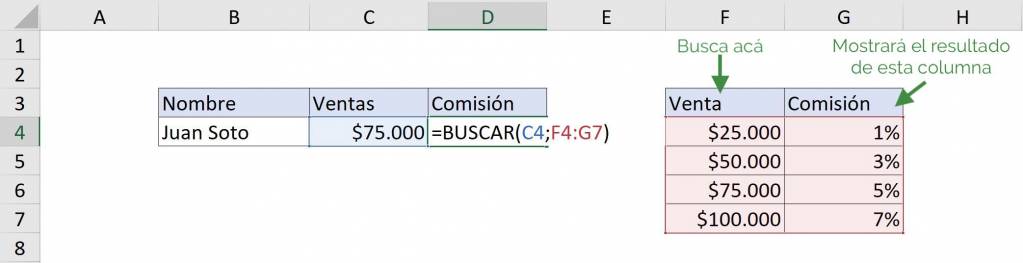
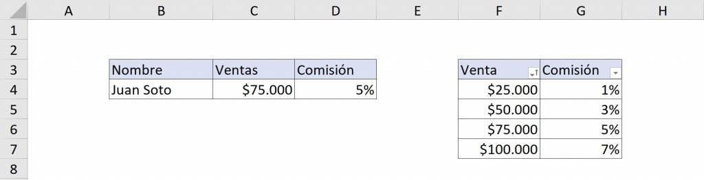
Let's look at a simple example to understand how SEARCH works. Here we want to find what commission corresponds to Juan Soto given his level of sales:

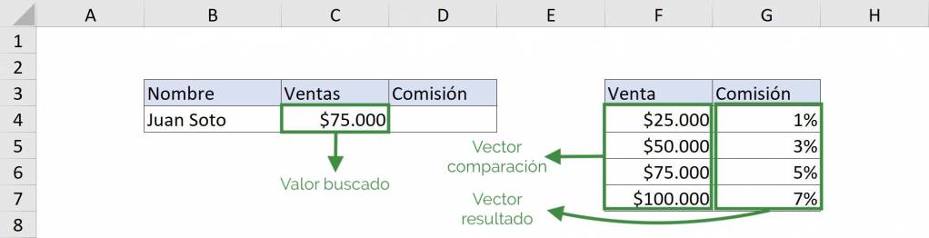
The elements that our SEARCH function must contain will be:

• lookup_value: C4
• comparison_vector: F4:F7
• result_vector: G4:G7

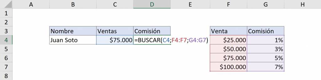
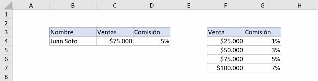
Thus, to use find the commission that corresponds to Juan Soto we must write “=SEARCH(C4;F4:F7;G4:G7)”. That way, We tell Excel to look for the value of cell C4 in the range of cells from F4 to F7 and that gives us as a result the value in the same position of the range from G4 to G7.

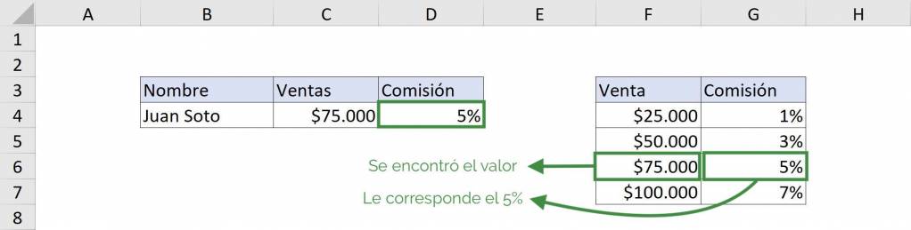
We finally obtain:

Ninja Tip: The SEARCH function is not case sensitive. For example, if we search for “Juan”, “JUAN” or “juan” will be found validly.

You can watch this video to complement your learning:

SEARCH function in matrix form

The SEARCH function is used to lookup a value from the first row or column and then return a value which is in the same position in the last row or column of the matrix:

• If the matrix covers an area that is wider than it is tall (more columns than rows), LOOKUP finds the value of lookup_value in the first row.
• If a matrix is square or taller than wide (has more rows than columns), LOOKUP searches the first column.

There are two very important factors when using the SEARCH function:

1. You must have organized lowest to highest vector values comparison (or alphabetically if values are text)
2. You must keep in mind that if the exact value is not found, An approximate value will be obtained downwards.

Let's look at the same example as in the previous section to understand how SEARCH works in matrix form. Here we want to find what commission corresponds to Juan Soto given his level of sales:

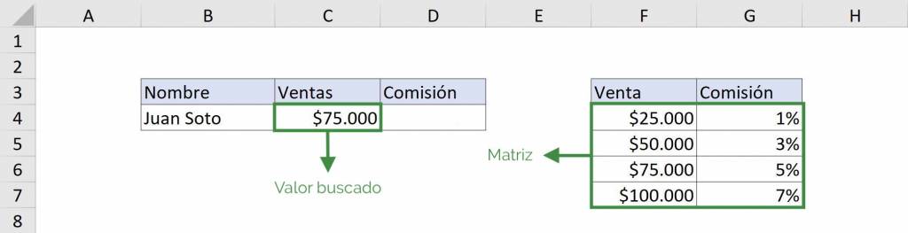
The elements that our SEARCH function must contain will be:

• lookup_value: C4
• matrix: F4:G7

Thus, to use find the commission that corresponds to Juan Soto we must write “=SEARCH(C4;F4:G7)”. That way, we tell Excel that find the value of cell C4 in the first column of the matrix (cells F4 through F7) and that gives us as a result the value in the same position of the last column of the matrix (range from G4 to G7).

Finally we obtain:

Ninja Tip: The LOOKUP function selects the last value in the row or column. If you want to specify a specific row or column you can use the functions HLOOKUP, VLOOKUP or XLOOKUP.

Rough SEARCH

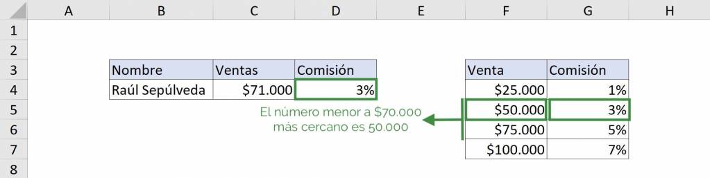
What happens when we have a value that is not within our data? If we take the previous example, what happens if someone has sales of $71,000? The SEARCH function will approximate “downwards”, that is, it will take the value minor closest that is in the table. In the following example we see:

Thus, if we have someone who has sales of $71,000 we have the same syntax: “=SEARCH(C4;F4F7;G4:G7)” or “=SEARCH(C4;F4:G7)”. In this case, the closest value less than $71,000 is $50,000 and the commission that corresponds to those sales is 3%:

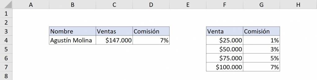
Ninja Tip: When we want to find a value that is greater than all the values in the search vector, The SEARCH function will assign the searched value that corresponds to the largest value of the vector. Thus, we can see in the following example of sales of $147,000, the commission that corresponds to $100,000 will be assigned.

Common errors in SEARCH

Do not sort data in ascending order

The function SEARCH searches “in order” from top to bottom or from left to right. In this way, by not having our data organized, Excel can give us the wrong result.

Let's look at the same previous example but now with the data out of order:

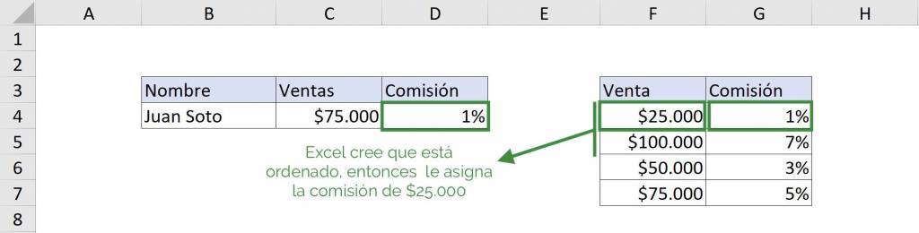
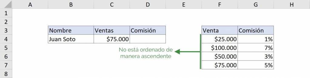In this way, when using the SEARCH function, the value $75,000 will be searched and Excel will assume that the data is ordered from largest to smallest. So, when you see $25,000 and then $100,000, Excel will believe that the next values in the table will be greater than $100,000. Therefore, the commission value corresponding to $25,000 is assigned because that is the closest minor value to $75,000 in the data. As we see in the image:

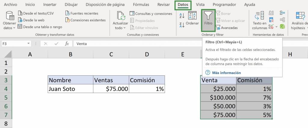
Ninja Tip: To easily sort the data we can select everything and apply a filter by going to the tab “Data” and then choose “Filters”. Next, we go to the “Sale” column of the table and press the down arrow and in the “Sort” section choose “Ascending”.

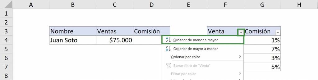
Thus, by having the data organized we get the correct result:

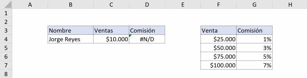
#N/D error in the SEARCH function

When we want to find a value that is less than all the values in the search vector, the LOOKUP function will return the value #N/D.

Thus, we can see in the following example of sales of $10,000:

Tip Ninja: complement and advance your learning by learning how to use the function VLOOKUP and VLOOKUP with multiple criteria.

​

Frequent questions