Excel VLOOKUP: Master the function in 3 steps

The function VLOOKUP It is by far one of the most popular features in Excel. In this post we will teach you how to master it in a simple way.

Key information:

VLOOKUP allows you to search for elements in a table. The elements that this function looks for must be to the right of the “lookup value”. Excel will look for the “searched value” in the first column of the range of cells (“table_matrix”) and will return the data from the column that you indicate in “column_indicator”. If you want to do an exact search you must enter 0 in the “range” parameter. If you want to do a rough search you must enter 1.

Tip Ninja: xLOOKUP It is an improved version of VLOOKUP and we recommend you use it. Unlike VLOOKUP and HLOOKUP it works in any direction, making it easier and more convenient to use than its predecessors. (*XLOOKUP is available for MS Office 365).

The basics:

Purpose: VLOOKUP allows us to search and find data in a specific column within a table, based on exact or approximate matches. It is especially useful for crossing databases that contain a large amount of information.
Characteristics: The letter 'V' in its name refers to the fact that the searches obey a vertical order. The search direction for this function is from our searched value column to the right.
Syntax: =VLOOKUP(lookup_value; table_array; column_indicator; [range])
Arguments:
- search_value: Value we want to search for.
- table_matrix: Range of cells in which we will search.
- indicator_columnas: Column that we want to obtain.
- [range]: Exact/approximate search.

Step 1: Understanding the VLOOKUP function

VLOOKUP finds data to the right

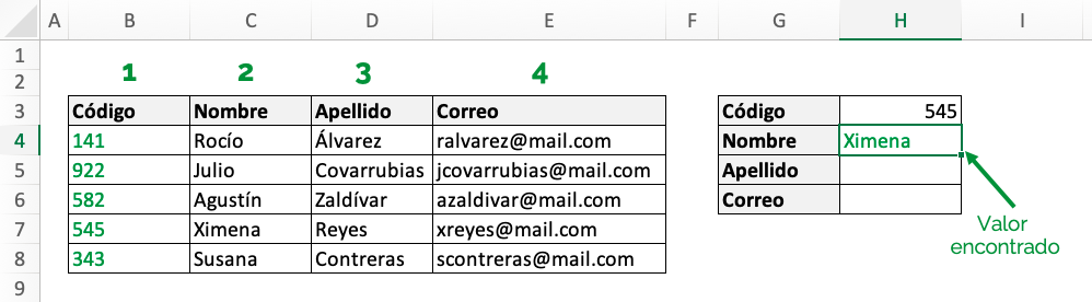
VLOOKUP allows you to find a value to the right of the “lookup value”. Taking the example of the following image, only with the code in cell H2 we could find the First Name, Last Name and Email of a person.

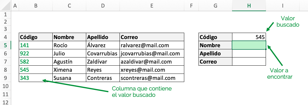
In the image we see that The value you want to find is the Name which corresponds to the code '545'. Therefore, since the 'Code' column contains the values we are looking for, VLOOKUP will search to the right, examining the 'First Name', 'Last Name' and 'Email' columns in our table.

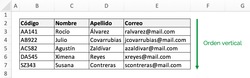
VLOOKUP searches vertically

The VLOOKUP function allows us to search and find values vertically, as shown in the image:

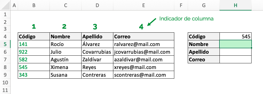
VLOOKUP gets data based on column indicator

When applying the Excel VLOOKUP function we must imagine that the columns of our table matrix are listed. In this case, if we wanted to find the value of 'First Name' our column indicator would be the number '2', if we wanted to find the 'Last Name' it would be the number '3', etc.

VLOOKUP allows us to search and find data based on two types of matches, exact and approximate. Let's see what each one is about.

Step 2: Using VLOOKUP with exact matches

To search with exact match we must enter 0 in the “range” parameter. In the following example we will search for the name of the person that corresponds to the code '545' in cell H5. Since the name of a person with the code 546 or 544 is not useful, we will perform a search with an exact match, and to do so we will enter 0 in the last parameter of the function.

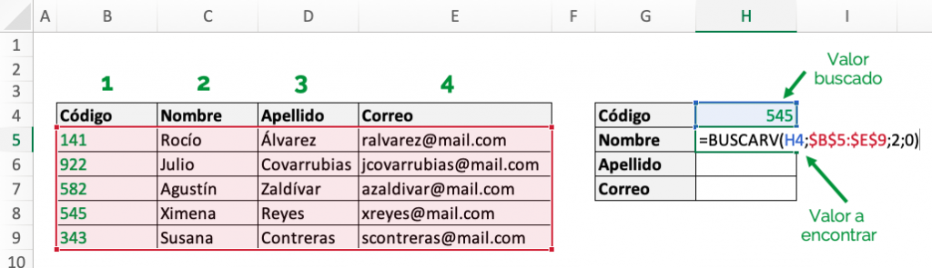
The elements that our VLOOKUP function must contain will be:

lookup_value = H4
table_array = $B$5:$E$9
column_indicator = 2 (“Name” column)
range = 0 (Exact match)

That is, our VLOOKUP function corresponds to:

=VLOOKUP(H4, $B$5:$E$9, 2, 0)

The result we obtain is:

We can see in our cell H5 that the name that the function returned is Ximena, which exactly matches the code '545' of our searched value.

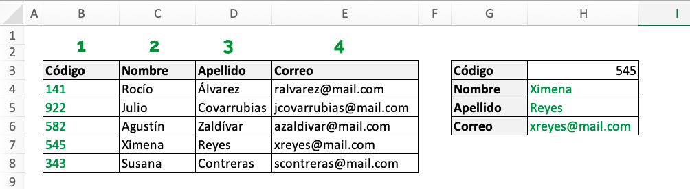
To obtain the last name and email of this person we would do:

=VLOOKUP(H4, $B$5:$E$9, 3, 0)

=VLOOKUP(H4, $B$5:$E$9, 4, 0)

With that, we would obtain the following result:

Step 3: Using VLOOKUP with fuzzy matches

To do searches with approximate match we must enter 1 in the “range” parameter. We will apply this option when we want to find the best possible match in the event that we cannot find an exact match. The use of approximate search is less common than exact search.

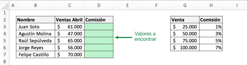
In the example below we want find the percentage of commission that corresponds to the sale made by each person. However, in the commission table there is no exact match for each of the amounts. Thus, we will use VLOOKUP with fuzzy matching to find the best possible match.

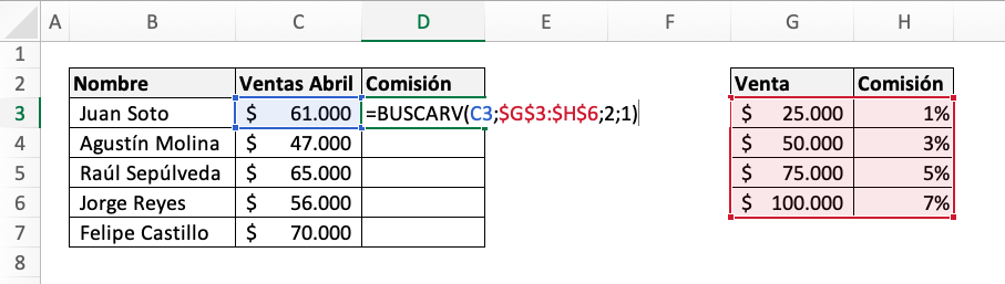
The elements that our VLOOKUP function must contain will be:

lookup_value = C3
table_matrix = $G$3:$H$6 (Fixed cell range because we will reuse the function)
column_indicator = 2 (“Name” column)
range = 1 (Fuzzy Match)

That is, our VLOOKUP function corresponds to:

=VLOOKUP(C3, $G$3:$H$6, 2, 1)

With this formula we obtain the following result:

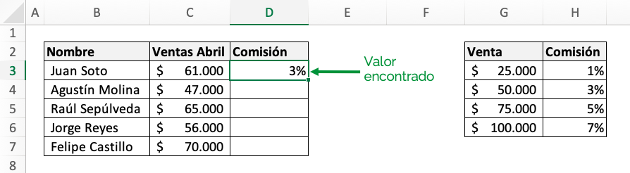
We can see in our cell D3 that the commission percentage that VLOOKUP delivers is 3%. Since it gives us the value of the amount larger smaller to $61,000, we see that the result is correct.

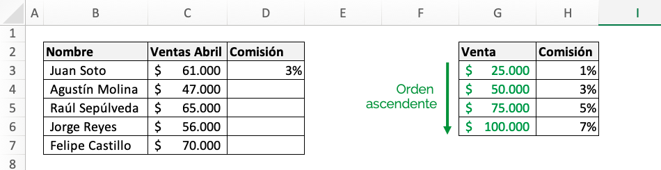
Ninja Tip: When using fuzzy matches in VLOOKUP, you should make sure the data is sorted in ascending order like the image below.

Common mistakes

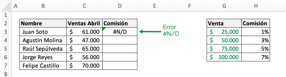
Error #N/D

When using VLOOKUP you may sometimes encounter the #N/D error. This error usually indicates that the function cannot find the searched value.

If this happens, we advise you to check the following points:

Check that the searched value exists in your table array and that it does not have typos.
Make sure that when entering your table matrix you have considered all existing columns.
Check that the indicator number of columns is correct.

Ninja Tip: If you do not want to show the errors in the table you can use the IF.ND or IF.ERROR formulas.

Are you interested in deepening your knowledge further? Let's move on then with:

VLOOKUP with multiple criteria

1. The basics of VLOOKUP with multiple criteria

What is VLOOKUP with m for?more than one criterion? It is used to find a specific piece of information, applying more than one rule.

What is the VLOOKUP function? It is a function that allows you to search for a specific data in a table, based on an indicated criterion. To know how to implement this excellent VLOOKUP function in detail, you can read this post.

But Can the VLOOKUP function do a search with more than one criteria?

No, the function itself does not allow it. BUT, there is a trick that does make it possible, through an auxiliary variable. In this way it is possible to search for data vertically and with more than one criterion.

2. VLOOKUP function with multiple criteria

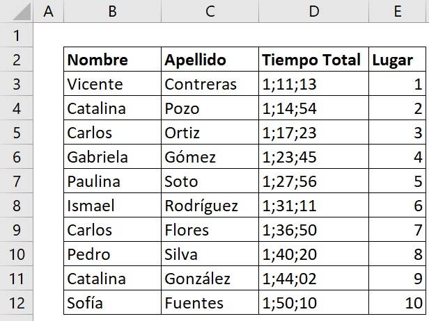
Let's imagine the following example of triathlon competitors. The following table shows the first name, last name, place and total time obtained in the competition for each of the players.

What do we do if we want to find the total time that Catalina González took in the competition? We apply the VLOOKUP function:

In search value, we put the cell with the name “Catalina”.
We select the range of the table where we are going to search for the previous value.
We indicate column number 3, since in that column the total times of the competitions are found.
Finally, we add the value zero because we want an exact value.

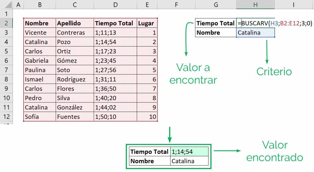
In this way, we find the total time it took to complete the triathlon: 1;14;54. But we see that this time does not correspond to that of “Catalina González” which is the one we are looking for, but to that of “Catalina Pozo”!

Why is this happening?

Because the VLOOKUP function returns the first searched value, which in this case the first one that appears in the table is that of Catalina Pozo.

Therefore, we must be more precise and indicate a second criterion, but the VLOOKUP function does not allow it.

How do we do it?

We create an auxiliary variable and apply VLOOKUP with multiple criteria.

3. Auxiliary variable

Through an auxiliary variable, we can join the search criteria we want. In this way, when VLOOKUP with multiple criteria, the function will not give us the first value, but rather the one we are really looking for.

In our example, the two criteria are first name and last name. Therefore, we create an auxiliary variable with these two components.

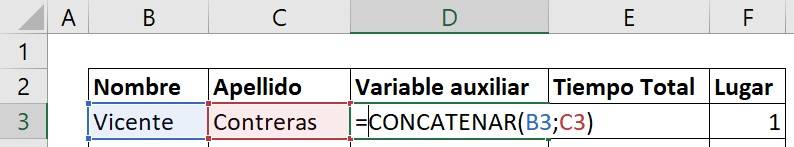
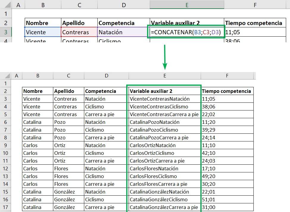
To create the auxiliary variable, we must concatenate the two variables. We can do this through the “&” sign, or with the CONCATENATE function.

In this case we will occupy the CONCATENATE function, as shown in the image below.

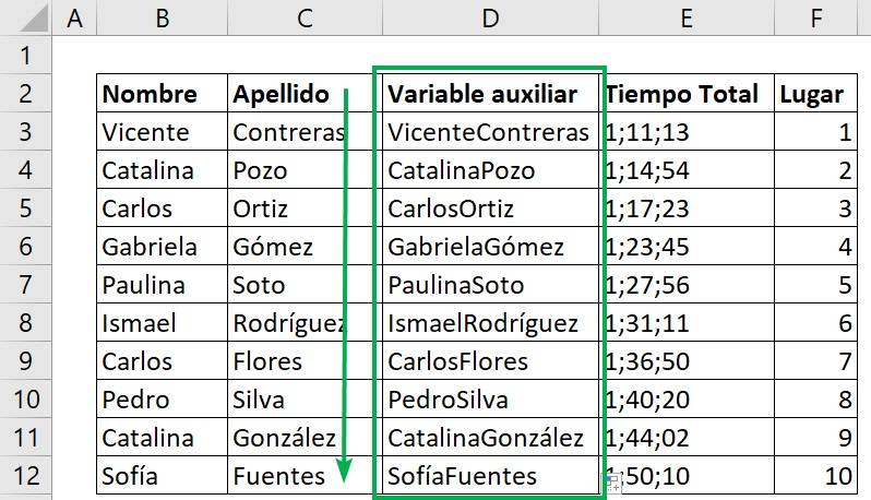
Thus we run downwards, obtaining the auxiliary variables for each of the competitors and thus being able to apply VLOOKUP with multiple criteria.

4. VLOOKUP with multiple criteria: 2 criteria

Once the auxiliary variable is created, we can VLOOKUP with multiple criteria, in this case there are 2.

How do we do it?

We apply the VLOOKUP function, but now in the first argument, we put the two criteria (name and surname) joined by “&”:

We define the new table range for VLOOKUP with multiple criteria

Ninja Reminder: In the VLOOKUP function the first column must contain the searched value. In this case it is the auxiliary variable with the names and surnames. So, that will be column 1 in the table range we selected for the function.

We write the column that contains the value to find. In this case it is column number 2.
We write “0” since we want exact matches.

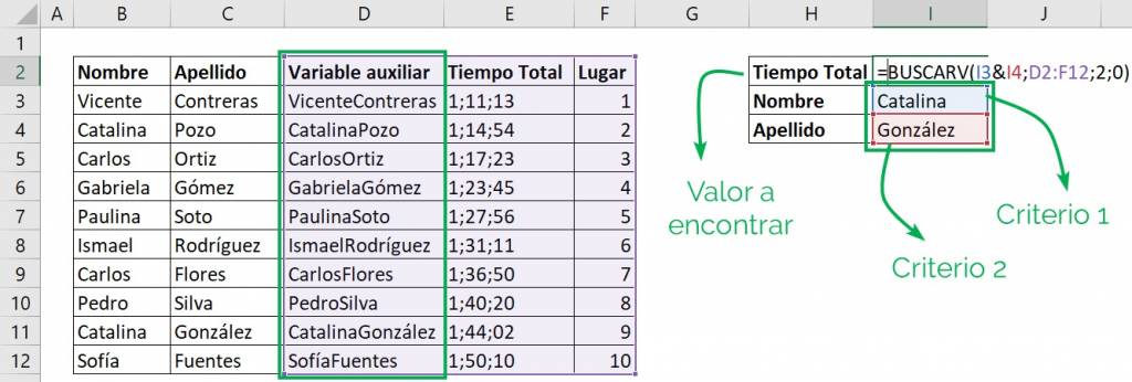
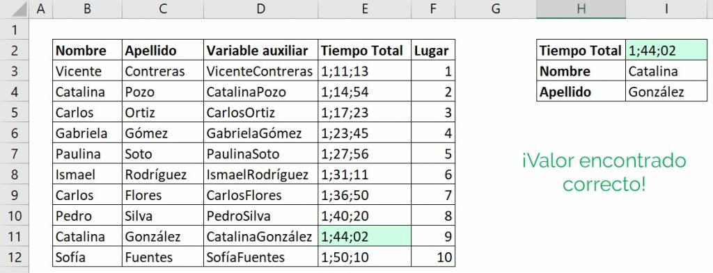
We apply the function and We see that now the function gives us the time of Catalina González, and not Catalina Pozo! Catalina González's time is 1;44;02, as can be seen in the following image.

We have already applied the VLOOKUP function with multiple criteria!

Likewise, we can apply this trick to any other triathlon competitor through VLOOKUP with multiple criteria.

Let's try for example for Carlos. We see that there are two competitors named Carlos; Ortiz and Flores.

If we want to find Carlos Flores' time, we simply change the first and last names in the lookup table, as we see below.

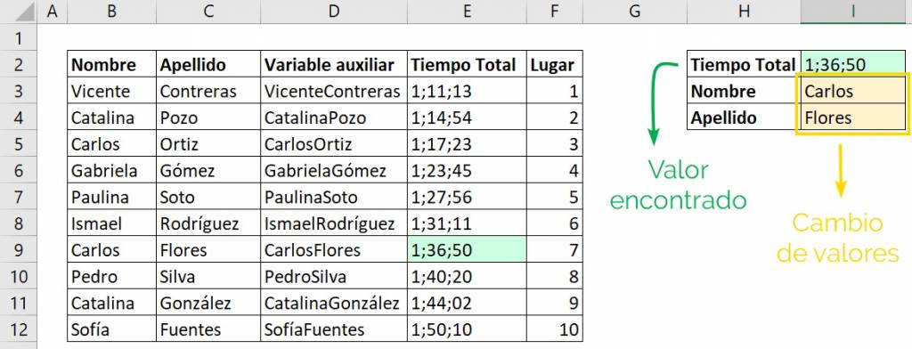
The time made by Carlos Flores is 1:36:50. We see that with this VLOOKUP trick with multiple criteria, the function gives us the value of Carlos Flores and not the first, which is Carlos Ortiz.

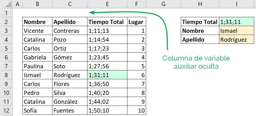
Even, we can hide the auxiliary variable column and the VLOOKUP trick with multiple criteria will continue to work for us.

In our example, if we now look for “Ismael Rodríguez”, we find that his time was 1:31:11, without needing to show the column of auxiliary variables.

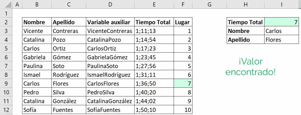
We can also change the VLOOKUP function with multiple criteria and instead of putting column “2”, we can put column “3”. This way we will know the place that the player obtained in the competition.

If we apply the above, we can see the case of Carlos Flores, who obtained number 7.

5. VLOOKUP with multiple criteria: more than 2 criteria

This trick allows us to do it with more than two searched values; 3, 4, or as many as we want.

How do we do it?

We must create an auxiliary variable with all the criteria we want to search for. If we want 3 criteria, we create an auxiliary variable with these three. If we want 4, we create a variable with those 4.

Let's imagine in our example that We also have the scores for each of the triathlon competitions: Swimming, cycling and running for some of the players, as shown in the image.

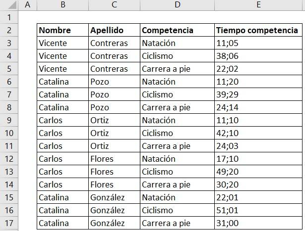
We see that as before, there are 2 Carlos and 2 Catalinas. But now There are 3 different competitions for each competitor. Therefore, if we search for the value “Catalina”, the VLOOKUP function will give us the first value.

In this case it would give us the Catalina Pozo's competition time in swimming.

So, to know the competition time of a player, in a specific competition, we need to add the last name and competition type in VLOOKUP with multiple criteria.

For this, We create an auxiliary variable as before, but this time with three criteria: First name, Last name and competence.

We concatenate these three variables, and run for all the rows, as seen in the following image in order to apply VLOOKUP with multiple criteria.

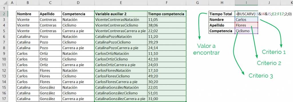
Now we apply the VLOOKUP function with multiple criteria:

In the first argument we join the three criteria through “&”.
We select the range of the table in which we will apply VLOOKUP with multiple criteria.
We indicate the column that contains the value to be found: column 2 in this case.
Finally we put zero, since we want an exact value and we press “Enter”.

We see that it gives us the value we were looking for! So we have applied VLOOKUP again with multiple criteria, but this time with 3.

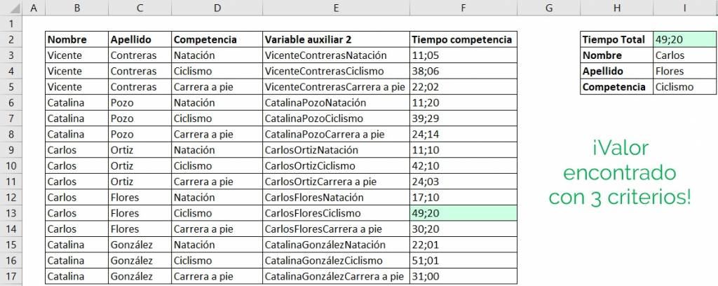
The time that Carlos Flores obtained in cycling was 49:20 minutes. And so we can iterate with the competitors and tests we want by applying VLOOKUP with multiple criteria!

Tip Ninja: There are other similar tricks like the MATCH or INDEX function, which you can look at in this post.

Excel VLOOKUP: Master the function in 3 steps

Key information:

The basics: