Loan Installment Calculation in Excel

In this article we leave you everything you need to know to calculate a loan fee in Excel.

1. The basics for calculating loan installments in Excel

How does a loan work?

A financial institution lends us an amount of money for a period of time, with an interest rate. But, we must return that amount of money along with the interest charged on the loan, how? We must pay a loan fee every period.

What is the loan installment calculation?

It is the calculation that we will carry out to know the amount of money that we will pay every period to return the amount of money that was lent to us.

What does the loan fee contain?

The loan installment is made up of the payment of interest, and the payment of the principal or loan (amortization).

We will make an amortization table to calculate the loan fee in Excel corresponding to each period. This way we can know the amount belonging to the interest payment and the amount belonging to the principal payment for each of them.

2. Amortization table for calculating loan installment in Excel

What is an Excel Loan Amortization Table?

It is a table that will indicate the payments that we will make every period to repay the credit.

To create the bank loan amortization table in Excel and be able to calculate the loan installment, we need the following data:

Credit amount (principal): how much money the financial institution lends us.
Interest rate: rate that the institution charges us for lending money, a way through which the financial institution obtains profits.
Number of payments (number of periods): How many payments we will make to return the money borrowed.

It is important to identify and organize this data in an Excel table.

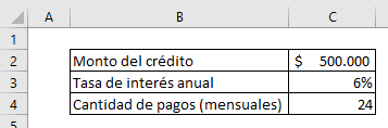
Let's imagine the following example with a credit amount of $500,000, which must be repaid in 24 monthly payments, with an annual interest rate of 6%. We write down this data in an Excel table as we see in the image.

Important data:

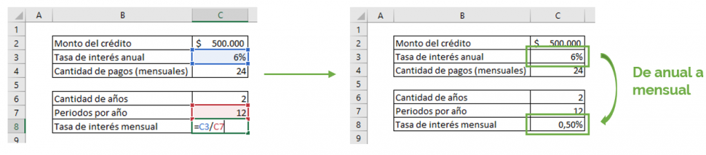
It's 24 months; It took us 2 years to pay the loan.
We must convert the interest rate to the corresponding period. They give us the annual interest rate, and the payments are monthly. Then we must change the annual interest rate to a monthly interest rate. As? We divide the rate by 12 as shown in the image, and we are left with the monthly interest rate of 0.5%. If they were semiannual payments, we divided them by 2, if they were quarterly payments, we divided them by 4.

What does an Excel credit amortization table look like?

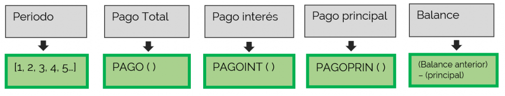
An amortization table to calculate the loan installment in Excel is made up of 5 elements:

The term
The total payment
Payment of interest
The payment of the principal
The balance

In this image you can see the 5 elements that make up the amortization table to calculate the loan installment in Excel. Each of these is associated with a function or formula, which we will see in detail below.

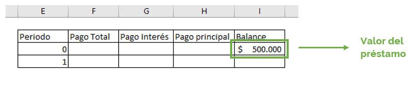
We will make the table with these 5 components in Excel as shown in the figure, which we will gradually complete.

3. PAYMENT function

The PAYMENT function calculates the amount of money that we will pay in each period. This payment is made up of the interest payment and the principal payment of our loan. The PAYMENT function is based on a constant interest rate and fixed payments over time.

Syntax: =PAYMENT(rate; nper; va; [vf], [type])

Arguments:

rate: credit interest rate (mandatory).
nper: number of total loan payments (mandatory).
va: current value; total sum of future payments accounted for in the present. It is the value of the loan today (mandatory).
[vf]: future value; balance that we want to leave after making the last payment. (Optional: if we do not put [vf], Excel sets future value equal to zero).
[type]: time when payments are due. It can be 1 or 0. [1]: at the beginning of the period, [0]: at the end of the period. (Optional: if we do not enter [type], Excel sets the payment due date for the end of the period).

If you want to learn more about the PAYMENT function, you can press the following link.

All elements of the PAYMENT function are always fixed. Then we set this data, as we see in the image.

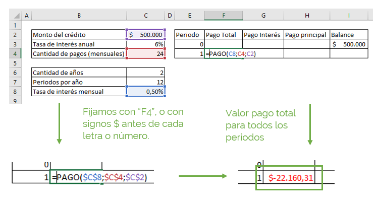
It's as easy as that, we have already done the loan installment calculation! The loan fee will be $22,160.31. We must pay this amount of money every month to return the credit they lent us.

4. PAGOINT function

The PAGOINT function calculates the part of the total payment corresponding to the interest payment for each period. It is a component of the loan installment calculation in Excel.

Syntax: =INTPAYMENT(rate; period; nper; va; [vf], [type])

Arguments:

rate: credit interest rate (mandatory).
period: corresponding period for which interest is calculated.
nper: number of total loan payments (mandatory).
va: present value: total sum of future payments accounted for in the present. The value of the loan today (required).
[vf]: future value; balance that we want to leave after making the last payment. (Optional: if we do not put [vf], Excel sets future value equal to zero).
[type]: time when payments are due. It can be 1 or 0. [1]: at the beginning of the period, [0]: at the end of the period. (Optional: if we do not enter [type], Excel sets the payment due date for the end of the period).

We set the rate, the number of payments, and the current value. The only thing we don't set is the period. For each period a different interest will be charged because the balance that remains to be paid changes.

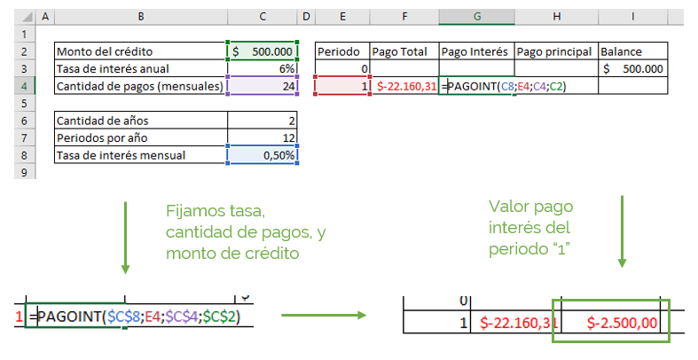
Only with this formula do we obtain the interest payment corresponding to period 1, that is, of the $22,160 that we will pay in the loan installment, $2,500 will be interest payments.

We can also calculate the interest payment by multiplying the interest rate by the previous balance amount, and it will give us the same thing.

5. PAGOPRIN function

The PAGOPRIN function calculates the part of the total payment corresponding to the principal payment for each period. It is a component of the loan installment calculation in Excel. In our example, we will see how much of the $500,000 that they lent us, we are going to pay in each period.

It occupies the same values as the PAGOINT function.

Syntax: =PAGOPRIN(rate; period; nper; va; [vf], [type])

Arguments:

rate: credit interest rate (mandatory).
period: corresponding period for which interest is calculated.
nper: number of total loan payments (mandatory).
va: present value: total sum of future payments accounted for in the present. The value of the loan today (required).
[vf]: future value; balance that we want to leave after making the last payment. (Optional: if we do not put [vf], Excel sets future value equal to zero).
[type]: time when payments are due. It can be 1 or 0. [1]: at the beginning of the period, [0]: at the end of the period. (Optional: if we do not enter [type], Excel sets the payment due date for the end of the period).

As in PAGOINT, we set the rate, number of payments, and credit amount. We leave the period variable, since the principal payment will be different in each period.

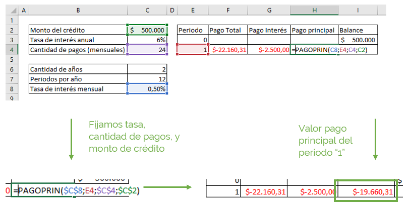
Thus we obtain that $19,660.31 will be the payment corresponding to settle the credit amount.

Of the $22,160.31 that we pay as a monthly loan fee, $19,660.31 belongs to the payment of the principal.
Of the initial $500,000 that we owed on the loan, we paid $19,660.31 in the first period, how much do we now owe on the total loan? Let's see how the balance is calculated below.

6. Balance of loan installment calculation in Excel

The balance or balance is the amount of money that we have left to return in each period of the credit amount, which can be calculated from the calculation of the Excel loan fee. It is calculated as follows:

In our example, we calculate that in period one, we paid $19,660.31. Therefore, from the initial $500,000 that we owed, we subtract the $19,660.31 to find out the new balance we owe, as we can see in the image. (We will add in Excel, since the “Principal Payment” already has the minus sign incorporated).

We do not set anything, since both the previous balance and the principal payment will change period to period.

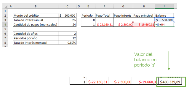This way we know that we still have to pay $480,339.69 of the $500,000 that they initially lent us.

7. Amortization table of all periods for calculating Excel loan installments

The credit amortization table will indicate in detail the calculation of the loan installment for each period. That is, it will show us the payments corresponding to; the total payment, interest payment, principal payment and balance for ALL periods.

How do we do it?

We simply repeat these steps for the next 23 payments that we have left to make, in what way? We select the range E4:I4 and drag down to period 24, that is, to row 27, as we see in the image.

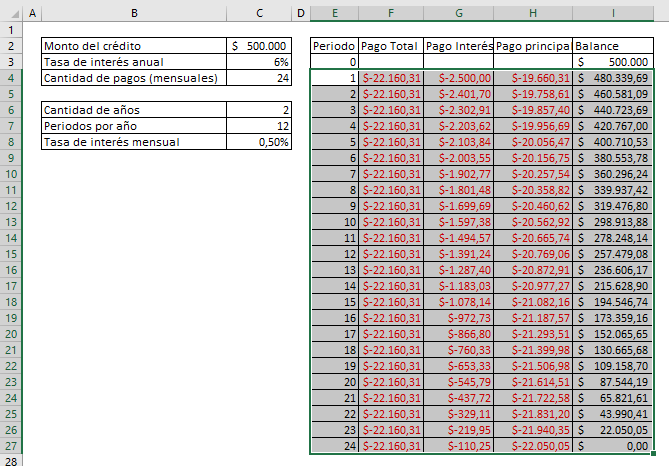
Calculating loan installments in Excel is that simple! We notice then how the interest payment, the principal payment and the balance vary from period to period, and how the value of the total payment is maintained. We see how in period 24 the balance is zero, that is, we owe $0, since we have paid our entire loan.

We notice that:

Decreases the interest payment.
The balance decreases, that is, after each period we owe less money.
Increase the principal payment.

Let's now see what happens if we decrease the number of total payments: from 24 to 12. We notice that the amount of the loan installment in Excel changes. We observe that the total payment increases, since we have fewer periods to pay the total debt, but the total amount of interest is lower.

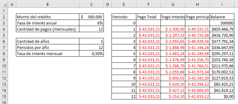
It is that simple to calculate the loan installment in Excel! What are you waiting for?

If you want to learn more about other financial functions, I recommend watching this post which talks about the CAGR function, which is used to find the compound annual growth rate of an investment.