INDEX: Master it in just 2 steps

The function INDEX Excel is a widely used tool because it provides the value found in a certain position. In this article you will learn to master it quickly.

Key information:

The INDEX function allows you to find values that occupy an exact position in a table or list, that is, this formula returns individual values.

Ninja Tip: The INDEX function can be used in conjunction with the MATCH function making the search for values faster and more dynamic, we recommend you visit INDEX and MATCH.

The basics

Purpose: The INDEX function allows us to find a value or text in an array by specifying the row and column number.
Characteristics: It can be used in two ways: array or reference. The array form allows you to search in one array, whereas the reference form allows you to search the value in more than one array.
Syntax:
- Array Form: =INDEX(array; row_num; [column_num])
- Reference Form: =INDEX(ref; row_num; [column_num]; [area_num])
Arguments:
- Matrix or ref: Range of cells where the data is located.
- row_num: Row number of the cell that has the value we are looking for.
- column_num: Column number of the cell that has the value we are looking for. This argument is optional if it is a list of values (only rows exist).
- area_num: number of the array in which the searched value is located.

Step 1: Using the INDEX function

The INDEX formula allows you to find values in a given position, specifying the row and column of the table or list of values. That is, it returns the value that intersects the given row and column.

Let's look at a simple example, we have a table with two columns and five rows. Through the INDEX function we can find any value. For example, we want to know which value is in row number “3” and in column number “2”.

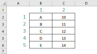
Tin Ninja: We must consider that the INDEX function lists the rows and columns according to the chosen data, so row “1” corresponds to the one with A and 1, that is, we should not be guided by the rows and columns of the Excel sheet.

In simple words, the INDEX function intersects the row and column number that we determined and responds to the value found at that intersection.

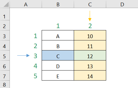
Therefore, as we look for row “3” and column “2”, Excel will intersect them and will respond with the intersected value, that is, the value found in the green cell.

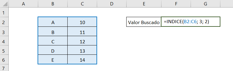
Since we are looking for row “3” and column “2”, the elements of the INDEX function will be:

matrix: B2:C7
row_num: 3
column_num: 2

That is, the INDEX function is:

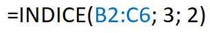
Therefore, the result we will obtain will be:

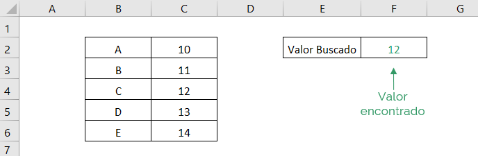
That is, the value found at the intersection of row “3” and column “2” is the number 12.

Step 2: Forms of the INDEX function

The Excel INDEX function allows you to search for data in a single array of values and also in multiple arrays. In the case of an array, the “array” argument is used; in the case of several arrays, we use the “reference” argument. Let's look at each case.

Matrix form

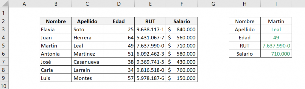
In the array form of INDEX, the first argument is the data array we use. For example, we want to know Martín's data, that is, know his Last Name, Age, RUT and Salary.

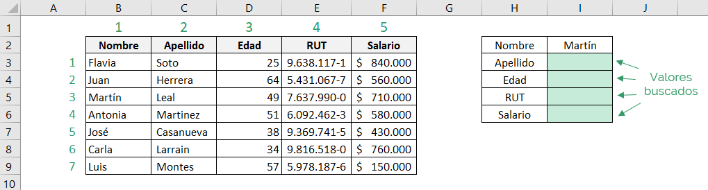
First, we will look for Martín's last name and then the other information. We see that the name Martín is in row number “3” and the surnames are in column “2”.

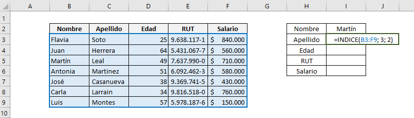
The elements of the function are:

matrix: B3:F9
row_num: 3
column_num: 2

That is, the INDEX function is:

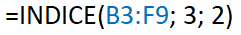
The result we will obtain will be:

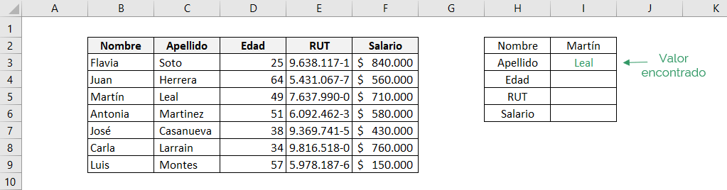
We can see in our cell I3 that the last name that the function returned is Leal, which exactly matches the name Martín.

To obtain Martín's age, RUT and salary, we must change only the searched column, since the row is still Martín's, therefore, we would do:

Age: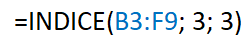

RUT: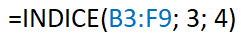

Salary: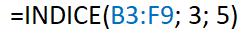

With that, we would obtain the following result:

We can see that the results obtained with the INDEX function coincide exactly with Martín's data.

Reference Form

This way of using the INDEX function allows us to evaluate more than one matrix at a time. In this case, the first argument, ref, will be all the corresponding data arrays.

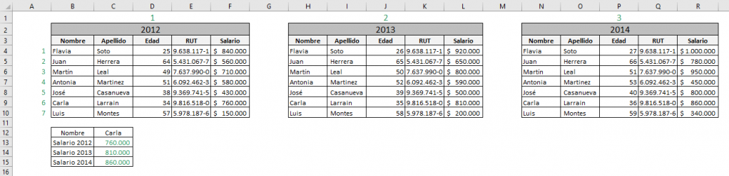
Continuing with the example, now we have the data for the same workers, but from different years. We want to know what Carla's salaries were in those years. Since each data table corresponds to one year, we have three matrices.

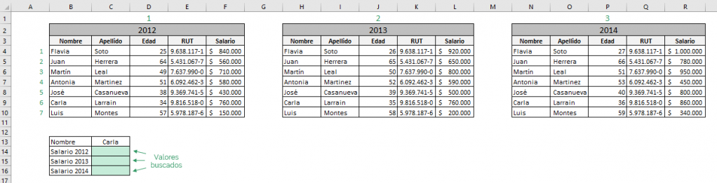
In this case, each matrix is equivalent to a number. Matrix 1 corresponds to the year 2012, matrix 2 to 2013 and, finally, matrix 3 corresponds to the year 2014. First we look for Carla's salary for 2012, therefore, the area_num argument corresponds to the number “1”.

Furthermore, since we are looking for Carla, the row number is “6” and since we are looking for salaries, the column corresponds to “5”.

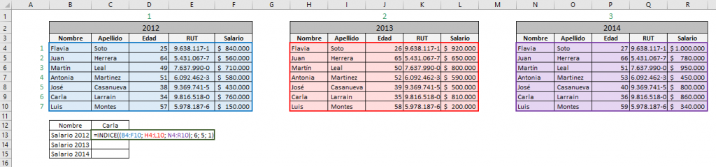
The elements of the function are:

ref: (B4;F10; H4:F10; N4;R10)
row_num: 6
column_num: 5
area_num: 1

Tip Ninja: It is very important that the matrices that we determine in the ref argument are enclosed in parentheses.

That is, the INDEX function is:

The result we will obtain will be:

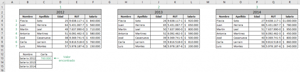
We can see that the salary that the function showed us exactly matches Carla's name in 2012.

To obtain the salaries of the other years, we must only change the area_num argument, as appropriate, since we are still in the same row and column, therefore, we would do:

2013:

2014:

With that, we would obtain the following result:

Common mistakes

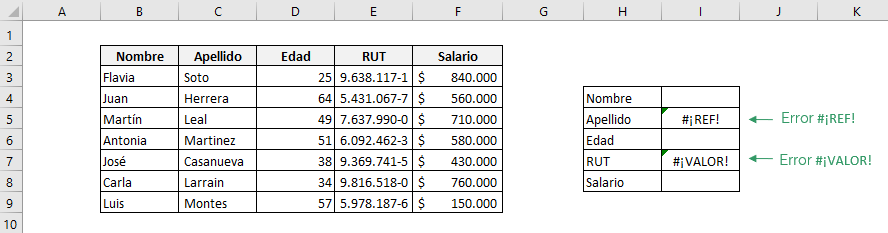
* #REF!

This error occurs when the arguments of the INDEX function indicate a cell that does not exist, that is, when the row or column number does not exist within the identified matrix or when the matrix number in the referential form does not exist. In this case, we recommend checking that the matrix number or the row or column number exist.

* #VALUE!

This error appears when the value of the row_num or column_num arguments is zero. The INDEX function only accepts values greater than 1 in these arguments.