Counting in Excel: count numbers, count cells, count everything

The Count function in Excel is widely useful, especially when we work with large databases. Review its many variations and advantages in this article.

Key information

Before starting, it is very important that you are clear about what you want to say in your Excel spreadsheet so that you can immediately go to the section of this post that will help you achieve your objective. 

Count cells with numbers

This function allows you to count those cells that contain only numbers 

• Syntax: COUNT(value1;[value2];…)
• Arguments: 
  • Value1: cell or range of cells to consider for counting. It is a mandatory element. 
  • Value2: Additional cell or range of cells to consider for counting. It's optional. 

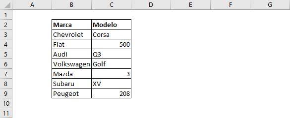
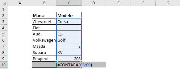
Let's try the following table containing makes and models of cars.

We will count the number of cells that have numbers: 

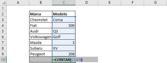
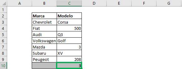
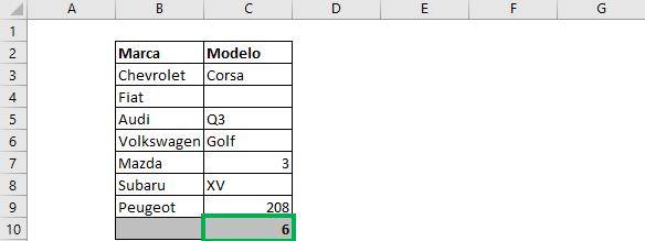
Make sure you select the entire range of cells where you want to count. The result is as follows: 

Note that this function counts the cells that contain only numbers. That is, even though “Q3” has a number, having a letter is considered a non-numeric cell. 

Count non-empty cells (with numbers or letters)

The function WILL COUNT allows you to count those cells that contain only numbers 

• Syntax: COUNT(value1;[value2];…)
• Arguments: 
  • Value1: cell or range of cells to consider for counting. It is a mandatory element. 
  • Value2: Additional cell or range of cells to consider for counting. It's optional. 

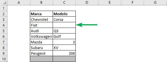
We will use the same table as before, but notice that now for “Fiat” there is no car model. 

We will now count the number of non-empty cells: 

Note that this command considers cells with any type of content except empty. The result is as follows: 

Count empty cells

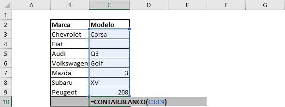
The function COUNTBLANK allows you to count those cells that have no content or are empty: 

• Syntax: COUNTBLANK(range)
• Arguments: 
  • Range: range of cells to consider for counting blank cells. 

The process is exactly the same as the previous case. We will take the same table whose model for “Fiat” is empty. 

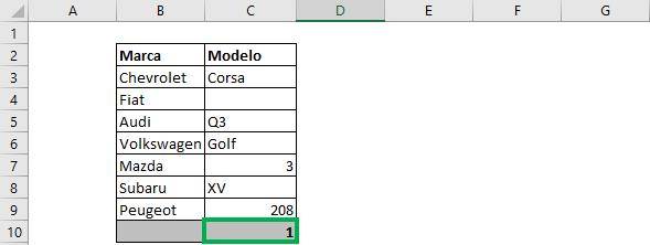
We count the empty cells: 

We see the result below: 

Have some condition

It is very common to want to count the cells that meet a certain condition. This can be numerical or text. 

The function COUNT YES will allow you to achieve this goal. We will now see a small example, but if you want to know more about this useful function, check the following article.

• Syntax: COUNTIF(range; criterion)
• Arguments:
  • range: the selection of cells in which to count
  • criterion: the condition according to which it will be counted

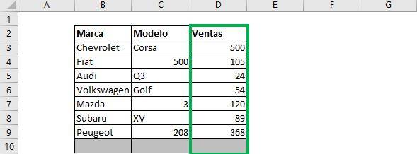
The table of cars with models now also includes a new column with the number of units sold, under the heading “Sales”. 

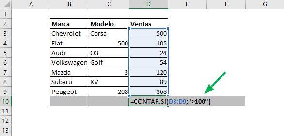
We will now count the number of models that have sales greater than 100. Note that since we are using a logical criterion (“greater than”), Excel needs it to be in quotes to know how to read it. Then, the formula looks like this: 

And when you press Enter, you get the following result: 

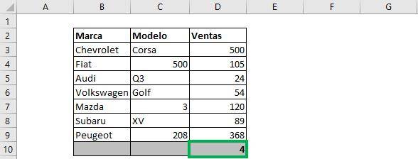
Which means that there are four models that have sales greater than 100. 

Unique values

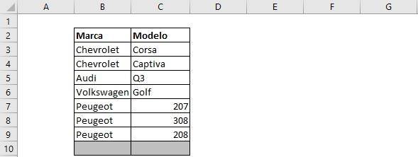
Many times a data set contains repeated data. This is not necessarily bad, but it can be a way to organize information correctly. For example, the table below again contains information about car brands and their respective models. We see that there are values that are repeated for “Brand”, but that are not repeated for model. That is, there are repeated values for “Brand” but there are no repeated values for the set “Brand” and “Model” (there are not two Chevrolet Corsa). 

Then, to count the unique values, simply enter the following formula: 

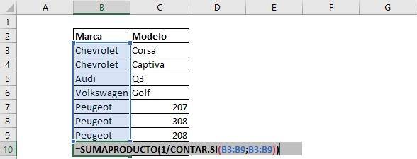
The most important thing is to note that you must take the same range twice, since we want to count the elements in “Brand”, considering the “Brand” criterion also to determine if the values are unique. The result is then the following: 

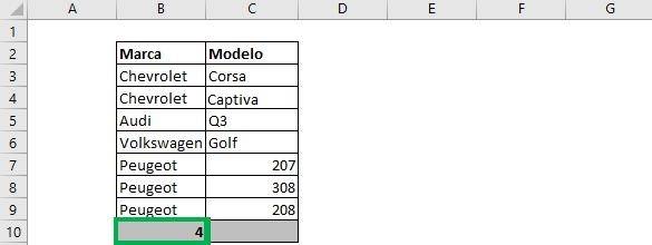
We see that there are 4 brands considered in the analysis, even though the table contains 7 rows of data. 

Ninja Tip: To count the unique values considering the Brand-Model pair, then you must make a new column that contains both elements. To gather the information into a single column, you can use the CONCATENATE function, and then use that new column as a range to count the unique values. 

Duplicate values

The opposite goal of counting unique values is to count duplicate values. This is naturally accompanied by identifying the number of duplicates according to category. 

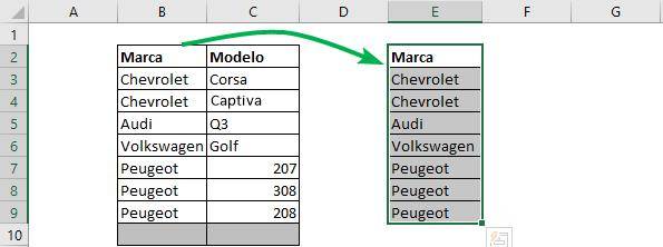
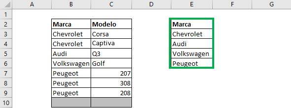
Step 1: Copy the “Brand” column to another part of the form and select its content. 

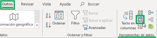
Step 2: Go to the “Data” tab, and in the “Data Tools” section, select the “Remove Duplicates” button. 

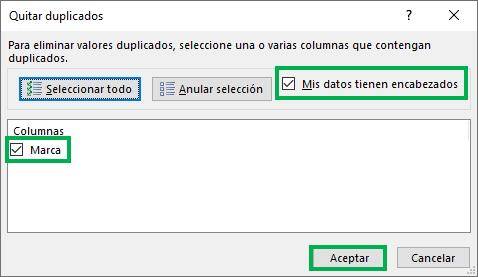
Step 3: A new window will appear. We see that it includes the option “My data has headers” and the section is for “Brand”. Simply click on “Accept”.

The result is a table that contains only the unique values. 

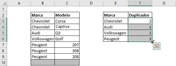
Step 4: Now we count the duplicate values. We need Excel to count all the times that the name of the Brand column (the duplicate) appears in the “Brand” column (the original). To do this, write down the following formula: 

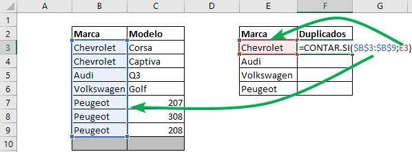
Make sure the “range” column where duplicates are searched is set to “$”. The result contains a 2, which is the number of times we found “Chevrolet” in the original “Brand” column. 

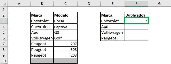
Step 5: Drag the formula down. We see that the number of duplicates it has now appears next to each mark. If “Duplicates” is greater than 1, then it is because the value appears more than once.