Test t Excel: learn how to apply it and test your skills

1. Test basics t Excel

What is t test?

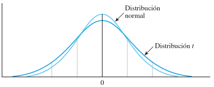
The Student T-test is a type of deductive statistics. It is used to analyze the behavior of two different samples.

What is the t test for?

T test Excel is used to analyze whether there is a significant difference between the means of two different samples.

Let's remember a couple of key concepts.

Hypothesis testing: It is a rule for accepting or rejecting a statement. To do this, it analyzes two opposing hypotheses of a population: the null hypothesis and the alternative hypothesis.

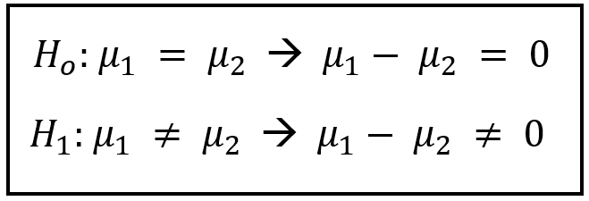
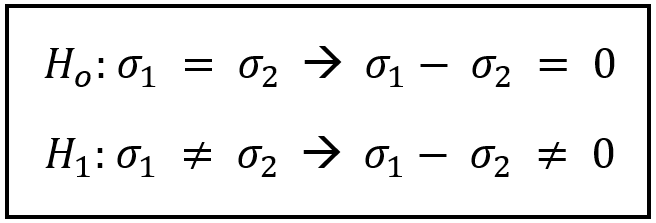
Null hypothesis (H0): guess about a parameter that you want to test. Generally the null hypothesis consists of the equality of a parameter in the two samples (absence of difference or effect). In the case of the Excel t test it is the equality of the means in two samples.

Alternative hypothesis (H1): conjecture of a parameter that is satisfied if the null hypothesis is rejected. It generally consists of the difference of a parameter in the two samples. For the Excel t test, there is a difference in the means of two samples.

We can see it in the image as follows:

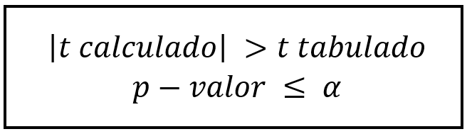
When is the null hypothesis rejected in an Excel t-test (H0)?

If the calculated t–Student absolute value (t statistic) is greater than the tabulated t (critical two-tailed t value).
If the p - value is less than the alpha of significance of the t-Student test. The p value is a measure of evidence against H0. If the above is true, there is sufficient evidence to reject H0. If it is not met, it is not statistically significant, and therefore H0 cannot be rejected.

Attention Ninja:

The Excel t-test works with the trusted 95% to perform your analyses, by default. Thus the alpha of an Excel t-test is 0.05.

You can perform the t test in Excel in three different ways:

Two-sample t test assuming equal variances.
Two-sample t test assuming unequal variances.
Paired two-sample t test.

The difference is due to the variances. To apply one or another option in a t-test in Excel, we must know how the sample variances behave. For this we must perform a Fisher test in Excel. The f test determines the equality of the variances of two samples (null hypothesis).

Therefore, once the f test is performed, we will be able to know the behavior of the variances and which of the t test methods to implement.

To apply the t test and the f test, we must load the “Data Analysis” plugin.

2. “Data Analysis” plugin for t-test in Excel

The “Data Analysis” tool allows you to perform different statistical, financial and technical analyzes through different instruments.

How is it loaded?

We go to “File”, click on “Options”. Then we select “Add-ons”, click on “Analysis Tools”, and press the “Go” key, as the image shows.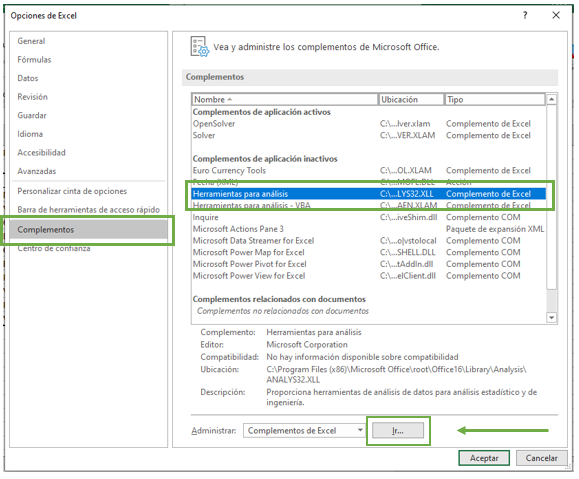We click on “Analysis Tools” and press “OK”.

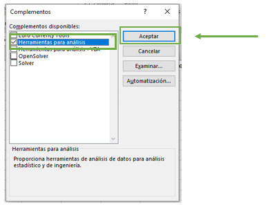
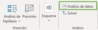
If we now go to “Data”, in the “Analysis” part, the “Data Analysis” add-on appears.

3. Excel t-test for two samples assuming unequal variances

The Excel t test allows you to compare the mean of two samples with different variances.

This post It could be useful if you are interested in knowing how to calculate the standard deviation in Excel.

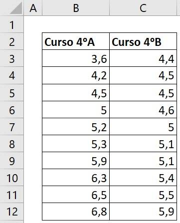
Let's imagine the following example where we have the grades of two courses, as shown in the table below.

The first step to perform an Excel t-test is to know if the variances of these two courses are equal. To do this we must perform an f test, with the null hypothesis and the alternative hypothesis being those shown in the image below:

How do we perform the Excel f test?

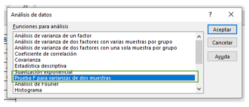
We go to “Data”, in “Analysis” we press “Data Analysis”.

We press “F test for two-sample variances”.

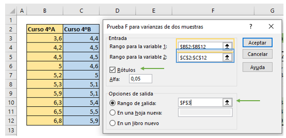
The following image box appears that we must fill out.

In range 1 we select the data from sample 1, in this case the notes from course 4A with the name of the sample.
In range 2 we select the data from sample 2, that is, the notes from course 4B with the name of the sample.
We click on “Labels”, since we have selected the name of each sample.
Excel's default alpha is 0.05, which we can change if we want. In this case we will leave it like this.
Finally we select the place where we want the table to appear on the current sheet. Excel also gives us the option of putting it on a new sheet, or a new workbook.

In this way, it gives us a table with the following analysis.

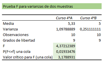
Let us remember that the null hypothesis in a Fisher test is rejected if any of these two conditions is met:

0.05 > 0.01933476
4.37212389 > 3.1788931

We see that both are true, therefore, the null hypothesis is rejected and the grade variances of the two courses are not equal.

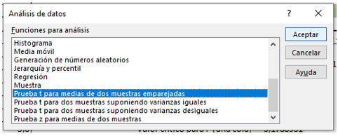
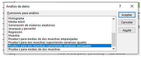
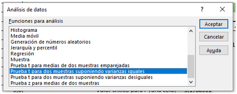
Now that we know this, we can perform the t-test. We go as before to “Data Analysis”, and now we select “T-test for two samples assuming unequal variances”.

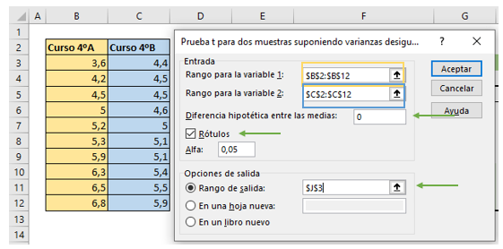
A box appears for the t-test very similar to the previous one, which we must fill in in a similar way.

In range 1 we select the data from sample 1, that is, the notes from course 4A with the name of the sample.
In range 2 we select the data from sample 2, in this case the notes from course 4B with the name of the sample.
We click on “Labels”, since we have selected the name of each sample.
Excel's default alpha is 0.05, which we can change if we want. In this case we will also leave it like this.
Finally we select the place where we want the table to appear on the current sheet. Excel also gives us the option of putting it on a new sheet, or a new workbook.

The difference will be that we must put a zero in “Hypothetical difference between the means”, since that is our null hypothesis of our t-test, that the means of the two courses are equal (that the difference between them is zero).

The following box appears for the Excel t-test:

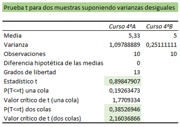
From this table we can test the null hypothesis of our Excel t-test, which is rejected if any of these two conditions are met:

0.05 > 0.38526946
2.16036866 < 0.89847907

We see that neither of the two is true, therefore, there is no significant evidence to say that the average grades of the two courses are different. The null hypothesis of our Excel t-test is not rejected.

4. Excel t-test for two samples assuming equal variances

Now suppose that a comparison of grades from course 4 A with course 4 C is made, as shown in the table.

We must see the behavior of the variances of these two samples to know which Excel t test we are going to perform.

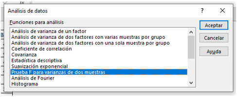
We go to “Data Analysis” and select “F-Test for Two-Sample Variances” just like before.

We fill in the data as in the previous example, as the image shows.

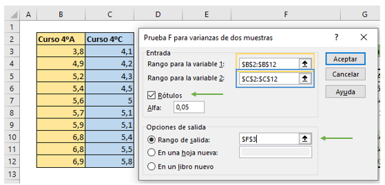
The following summary table appears.

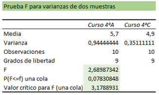
The null hypothesis in a Fisher test is rejected if either of these two conditions is met:

0.05 > 0.07830848
2.68987342 > 3.1788931

We see that the above is not true, and therefore the null hypothesis is not rejected, since there is no significant evidence to say that the variances of the grades of the two courses are different. Equal variances of the two courses are assumed.

In this way we go to “Data Analysis” and select “T-test for two samples assuming equal variances”.

We fill in our Excel t-test data just like before, as the image shows.

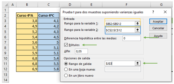
The following summary table of our Excel t-test appears.

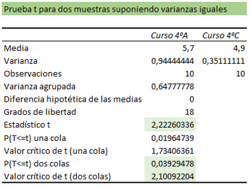
With this table we can test the null hypothesis of our Excel t-test, which is rejected if any of these two conditions are met:

0.05 > 0.03929478
2.10092204 < 2.22260336

We see that the above is true, therefore, the null hypothesis of our Excel t-test is rejected, that is, the averages of the grades of the two courses are different.

5. Excel t-test for paired two-sample means

This Excel t test deals when there is not complete independence between the samples. For this test the variables must have the same number of observations.

It is performed in a similar way as the two tests described above, but this time we will check the “T-test for paired two-sample means” option, as the image shows without having to do an Excel F-test first.