INDEX and MATCH: learn to use them easily

The functions INDEX and COINCIDE Excel are very popular tools since they allow you to search for elements in a table or range and they can also be combined. In this article you will quickly learn how to use them separately and also together. 

Key information:

The INDEX function allows you to find values that occupy a position in a table or list. The MATCH function returns the relative position that a value occupies within a list. By using both functions together, you will become a true Excel Ninja.

Ninja Tip: In addition to the INDEX and MATCH functions, we recommend another Excel tool that allows you to search for values in a data array, the famous function VLOOKUP. 

INDEX function

The Excel INDEX function allows you to find values in a data matrix by determining the row and column, that is, it returns the value that is in the position we ask for. 

For example, if we have the income and expenses of a company, we can easily and quickly search for what the expenses were for the month of May.

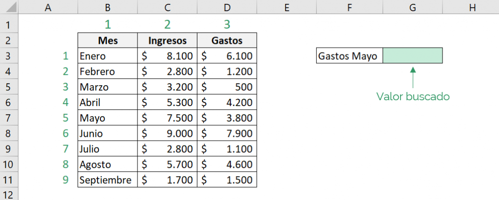
Since it is the month of May, we want Excel to search in that row, therefore, it is row number “5”. We also look for the expenses, which correspond to column three, therefore, the column is number “3”. 

Remember that Excel puts imaginary numbers in the selected matrix, so we should not be guided by the numbers of the rows or columns of the Excel sheet. 

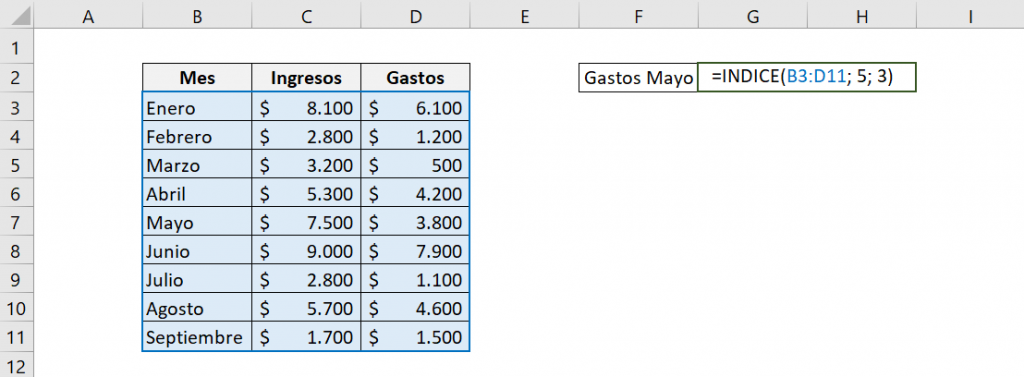
So, the elements of the function are:

• matrix:B3:D11
• row_num: 5
• column_num: 3

That is, the INDEX function is:

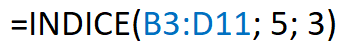
The result we will obtain will be:

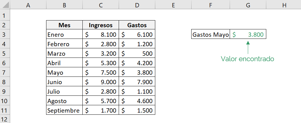
We can verify that the May expenses correspond to the result delivered by Excel. 

If you want to learn more about this function, we recommend visiting the formula blog INDEX.

MATCH function

The function COINCIDE Excel allows us to find the numerical position of an element in a list of values, that is, Excel gives us the number of the position in which the searched value is. 

There are three types of matches, exact match, less than and greater than. If you want to learn more about this feature and how to handle match types, we recommend visiting the MATCH feature.

Continuing with the example, we want to see what was the month in which there was income of $7,500. For this, we must use the “exact match” match time.

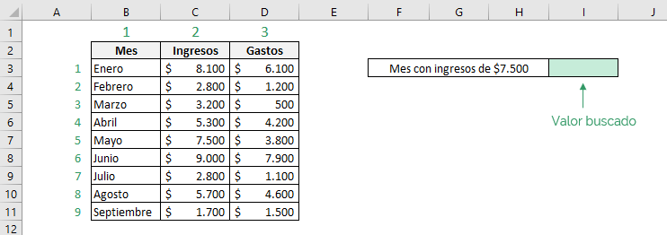
Since we are looking for the income, we must tell Excel that only that column is used, then the searched matrix corresponds to the income column. Also, since it is an exact match, the match_type is “0”.

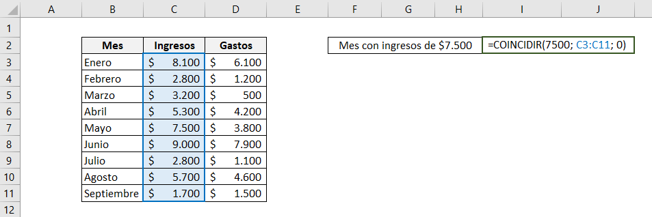
The elements of the function are:

• search_value: 2800
• search_array: C3:C9
• match_type: 0

That is, the MATCH function is:

The result we will obtain will be:

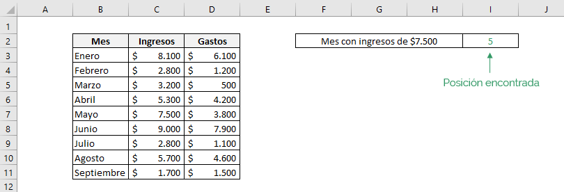
We can verify that position number 5 in the income column is the row for the month of May, that is, the month in which there was $7,500 in income was May. 

Combine the INDEX and MATCH functions

By using both functions together you will become a true Excel ninja. This tool allows you to find values more quickly and dynamically in a database.

To combine them correctly, we must include the MATCH function within the INDEX function. The MATCH function can be used on the number of rows, the number of columns, or both arguments of the INDEX function. Let's look at each case.

MATCH determines the row that uses INDEX

In this case, the MATCH function will determine the row that the INDEX function should search, that is, it will be found in the row_num argument.

For example, we want to find out what the expenses were for the month of April.

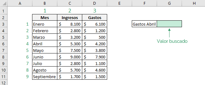
For this, the MATCH function looks for the value called “April” in the list of months. Furthermore, we are faced with an exact match, so in the match_type argument we must write a “0”. Also, since we are looking for expenses we must indicate that it is column number 3.

Remember that since we are looking for a text value, it must be enclosed in quotes. 

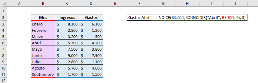
The elements of the function are:

• matrix: B3:D11
• row_num: MATCH function:
  • search_value: "April"
  • search_array: B3:B11
  • match_type: 0
• column_num: 3

That is, the INDEX function is:

The result we will obtain will be:

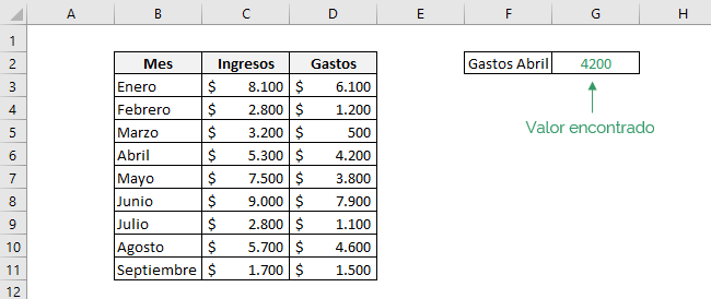
We can see that the result delivered by Excel coincides with the expenses generated in April.

MATCH determines the column that uses INDEX

In this case, the MATCH function will determine the column in which the INDEX function should search, that is, it will be found in the column_num argument.

For example, we want to find what the income was for the month of September.

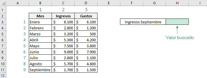
For this, the MATCH function looks for the value called “Revenue” in the category row, and we are also faced with an exact match, that is, the match_type argument is “0”. Also, since we are looking for the month of September, it corresponds to row number “9”.

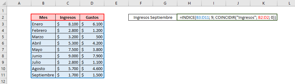
The elements of the function are:

• matrix: B3:D11
• row_num:  9
• column_num:  MATCH function:
  • search_value: "Income"
  • search_array: B2:D2
  • match_type: 0

That is, the INDEX function is:

What it means is: “MATCH will tell you which column the income is in and then INDEX will intersect that column with row 9.”

The result we will obtain will be:

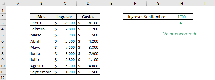
We can see that the result delivered by Excel coincides with the income generated in September.

MATCH determines the row and column that INDEX uses

In this case, the MATCH function will determine the row and column in which the INDEX function should search, that is, it will be found in the row_num and column_num argument.

For example, we want to see what the expenses were for July.

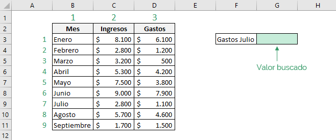
For the row number, the MATCH function will look for the value “July” and for the column number, the second function will look for the value “Expenses”. In both functions we use the exact match type. 

The elements of the function are:

• matrix: B3:D11
• row_num:  MATCH function:
  • search_value: "July"
  • search_array: B3:B11
  • match_type: 0
• column_num:  MATCH function:
  • search_value: "Bills"
  • search_array: B2:D2
  • match_type: 0

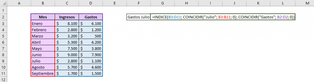
That is, the INDEX function is:

What it means is: “First, MATCH will tell you which row the month of July is in. Second, it will tell you which column the expenses are in. Finally, INDEX will intersect the row and column, delivering the corresponding result.

The result we will obtain will be:

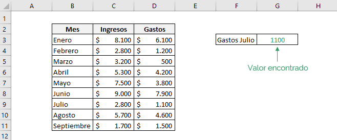
We can see that the result delivered by Excel coincides with the expenses generated in July.

Common mistakes

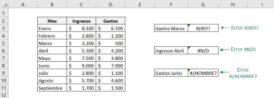
* #REF!

This error occurs when the arguments to the INDEX function indicate a cell that does not exist. In this case, we recommend checking that the row or column number exists. 

* #N/D

This error occurs when the MATCH function does not find a match. 

* #NAME?

This error usually indicates that there is an error in the MATCH formula. We advise you to review the following points:

1. Check that if the searched value is text, that it is enclosed in quotes. 
2. Make sure the searched value exists in the list of values.

Ninja Tip:  You can use the IF.ERROR or IF.ND functions to handle errors.

If you have any questions, we recommend the following video that shows how the INDEX function works, the MATCH function and how both work together.

Do you still have doubts about the MATCH function?…

MATCH: learn to use it quickly

The function COINCIDE Excel is a very popular tool because it provides the position occupied by a given element in a list of values. In addition, this formula offers three types of matches. In this article you will learn how to use it quickly.

Key information:

The MATCH function allows you to find the relative position of a value in a row, column or table, that is, this formula searches for an element and gives us its position.

Ninja Tip:  Generally the MATCH function is used in conjunction with the INDEX function, making the search for values faster and more dynamic, we recommend you visit INDEX and MATCH.

The basics

• Purpose: The MATCH function allows you to find the relative position of a searched value in an array of values.     
• Characteristics: This function allows three ways to search: with an exact match, major or minor.
• Syntax: =MATCH(lookup_value; lookup_array; [match_type])
• Arguments:
  • search_value: Value or text that we want to find. 
  • search_matrix: Range of cells where the values are found.
  • [match_type]: Specifies how Excel matches the lookup_value in the lookup_array. There are 3 types: exact match, less than and greater than. This argument is optional, if not set, Excel will do a “less than” match automatically.

Using the MATCH function

Excel's MATCH function allows you to find the relative position of a searched value in a given row, column, or table of values. 

To better understand how MATCH works, let's look at a simple example. We have a table with two columns and five rows. Through the function, we can find the position of any value. For example, we want to know what the position of the letter “D” is. 

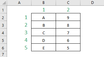
Tin Ninja: We must consider that the MATCH function lists the rows and columns according to the chosen data, so row “1” corresponds to the one with A and 9, that is, we should not be guided by the rows and columns of the Excel sheet.

In simple words, the MATCH function will search for the value in the given range of values from top to bottom, answering the position it is in. 

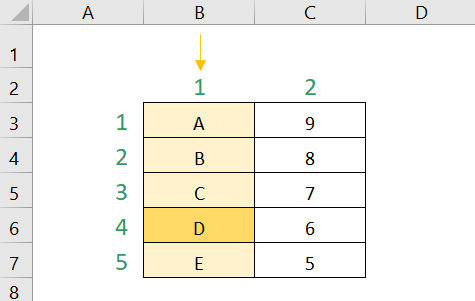
Therefore, as we are looking for the element “D” we must indicate that the letters are in column “1”, Excel will look for “D” in column “1” from top to bottom and will tell us the position in which it is located. .

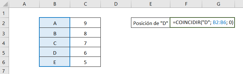
Then, the elements of the MATCH function will be:

• search_value: “D” 
• search_array: B2:B6 
• [match_type]: 0

Tip Ninja: If he search_value It is a text value, we must write it in quotes, otherwise Excel will not recognize it. 

Therefore, the result we will obtain will be:

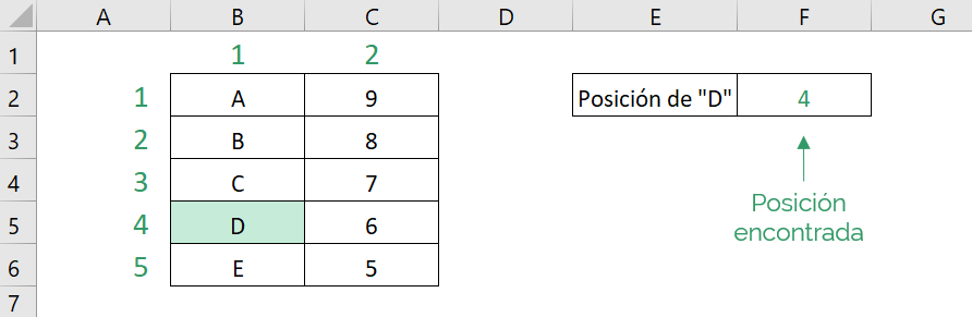
That is, element D is positioned in row number “4” of the letter column.

Excel's MATCH function offers three types of matches, making the search more flexible, these are: exact match, less than and greater than. We can also do a rough search. Let's look at each case.

Exact match

For this type of match we must write a “0” in the argument match_type. Excel will find the first value that is exactly the same as the searched value. 

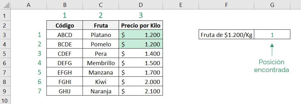
For example, we want to know which fruit has a price of $2,000 per Kilo. 

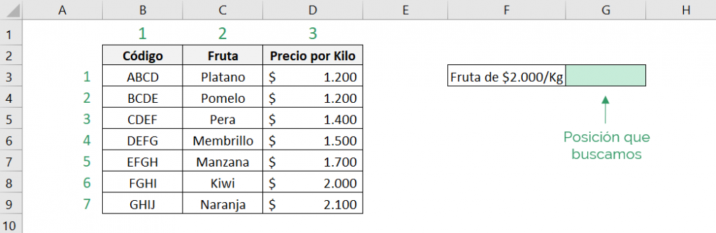
Since we are looking for the price per kilo, we must select the matrix that contains only the prices.

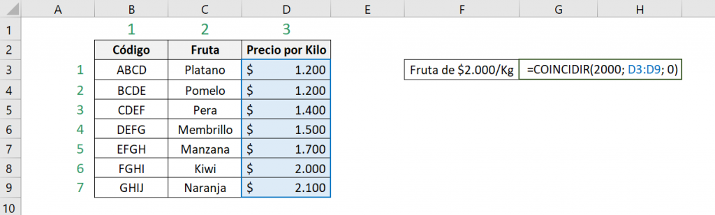
The elements of the function are:

• search_value: 2000
• search_array: D3:D9
• match_type: 0

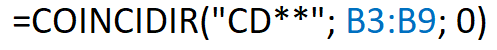
That is, the MATCH function is:

The result we will obtain will be:

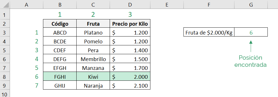
We see that the fruit that has a price of $2,000/Kg is in row number “6”, therefore, the kiwi is the fruit that has a price of $2,000 per kilo. 

What happens if there are two fruits with the same price? Which position does Excel respond to? The MATCH function returns the first exact match it finds. For example, banana and grapefruit have the same price per kilo, $1,200, but since the first value $1,200 is in row “1”, Excel will respond 1. 

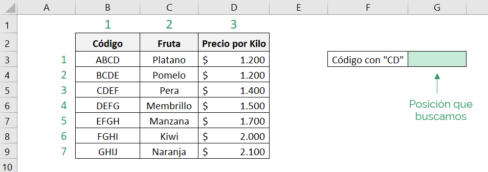
Exact match with wildcard

When we set an exact match type we can use wildcards. A wildcard is a special character that allows similar matches to be made. Excel interprets the wildcard “?” as any character and interprets the wildcard “*” as any sequence of characters, this allows us to perform searches with some specific values.   

For example, we want to look for a fruit code that starts with “CD” but we don't care about the other elements, this means that Excel should look for the code that starts with “CD” regardless of the rest of the code. 

Since all codes have 4 values and we only want the first two, the search_value It will be as follows “CD**”. 

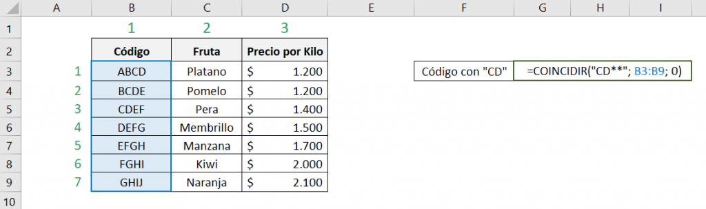
The elements of the function are:

• search_value: “CD**”
• search_array: B3:B9
• match_type: 0

That is, the MATCH function is:

The result we will obtain will be:

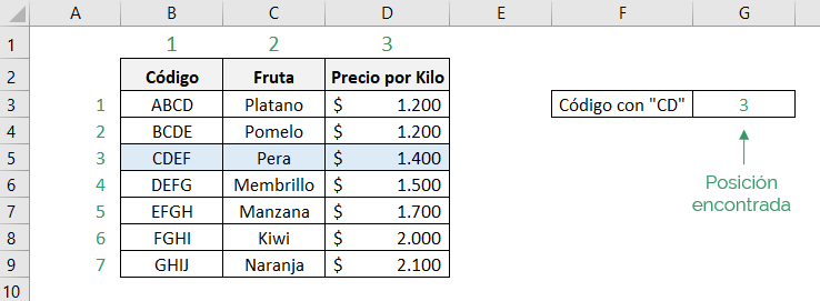
Therefore, the fruit that has the code starting with “CD” is the pear. 

Smaller than

For this type of match we must write a “1” in the argument match_type. Excel will find the first value that is less than or equal to the searched value. For this match, the list of elements must be sorted in ascending order, that is, from smallest to largest.

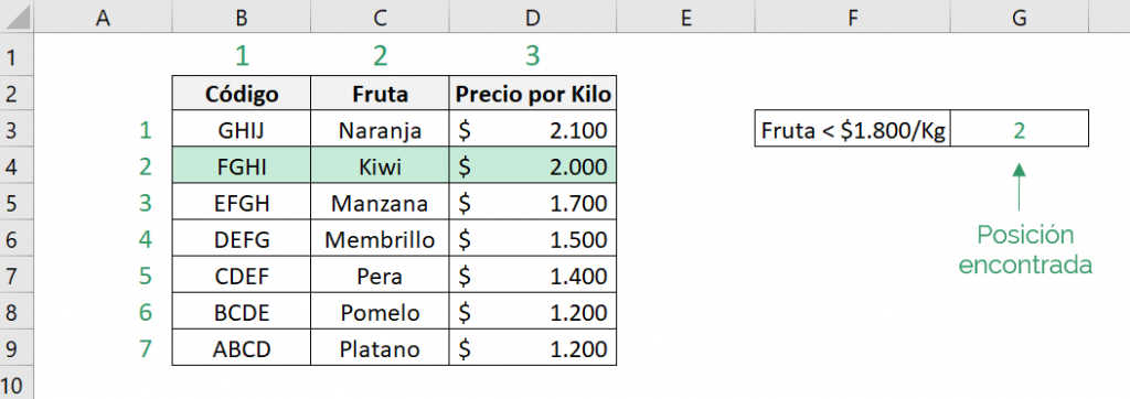
For example, we want to know which fruit has a price less than $1,800 per kilo.

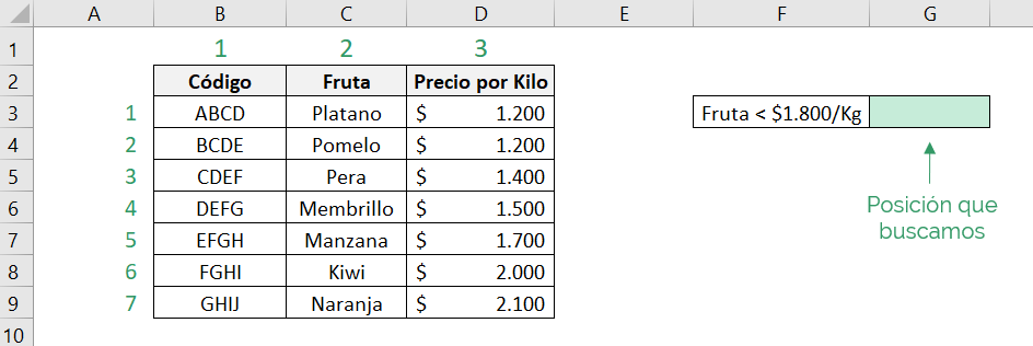
Since we are looking for a price less than $1,800 per kilo, we must select the column that contains only the prices.

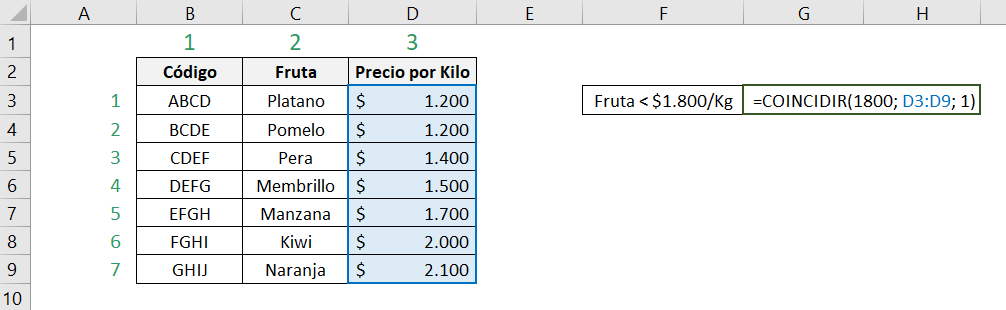
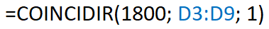
The elements of the function are:

• search_value: 1800
• search_array: D3:D9
• match_type: 1

That is, the MATCH function is:

The result we will obtain will be:

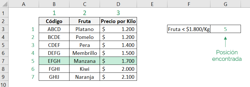
Excel answered position 5, that is, the apple is the fruit that has a price per kilo less than $1,800. We can see that the apple is not the only fruit with a price lower than $1,800, but Excel will respond to the first value that is closest to the determined one.

Greater than

For this type of match we must write a “-1” in the argument match_type. Excel will find the first value that is greater than or equal to the searched value. For this match, the list of elements must be sorted in descending order, that is, from largest to smallest.

For example, we want to know which fruit has a price higher than $1,900 per kilo.

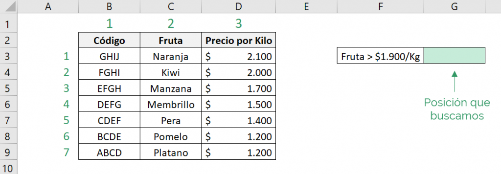
Since we are looking for a price greater than $1,900 per kilo, we must select the column that contains only the prices.

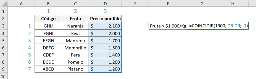
The elements of the function are:

• search_value: 1900
• search_array: D3:D9
• match_type: -1

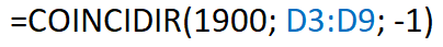
That is, the MATCH function is:

The result we will obtain will be:

Excel answered position 2, that is, kiwi is the fruit that has a price per kilo greater than $1,900. We can see that kiwi is not the only fruit with a price lower than $1,800, but Excel will respond with the first value that is closest to the determined one.

Fuzzy search

The MATCH function also allows fuzzy searches. For this, we use the less than match. For example, we want to search for a code similar to “CTOF”.

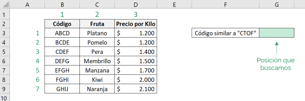
Since we are looking for a code we must select only that column, without including the fruit and the price.

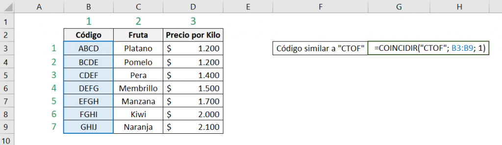
The elements of the function are:

• search_value: “CTOF”
• search_array: B3:B9
• match_type: 1

That is, the MATCH function is:

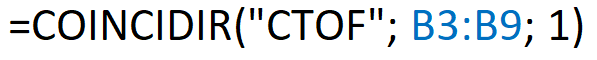
The result we will obtain will be:

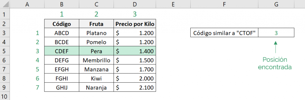
Excel searched for a fuzzy match by returning the code CDEF, which is only two letters different from CTOF.

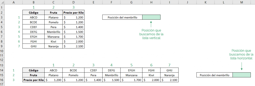
Horizontal and vertical matrix

Excel's MATCH function can be used on vertical and horizontal arrays. For example, if we want to know what position the quince occupies in the list of fruits, we will obtain the same result if the list is vertical or horizontal.

Since we are looking for quince, we are faced with an exact match. Additionally, since it is a text search, we must write it in quotes so that Excel can recognize it.

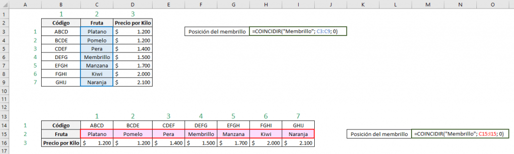
That is, the MATCH function is:

In the vertical list: 

In the horizontal list: 

The result we will obtain will be:

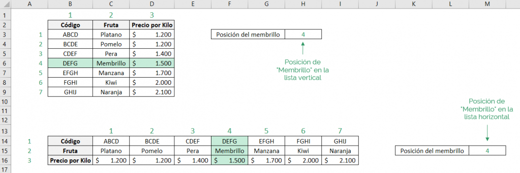
We can see that in both lists we obtain the same relative position of the quince.    

Common mistakes

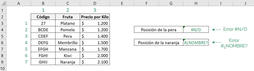
* #N/D

This error occurs when the MATCH function cannot find any matches or when the selected matrix is not a single row or column.

* #NAME?

This error usually indicates that there is an error in the MATCH formula. We advise you to review the following points:

1. Check that if the searched value is text, that it is enclosed in quotes. 

2. Make sure the searched value exists in the list of values.

Ninja Tip:  You can use the IF.ERROR or IF.ND functions to handle errors.