Find and remove duplicates in Excel: learn in 3 steps

Key information

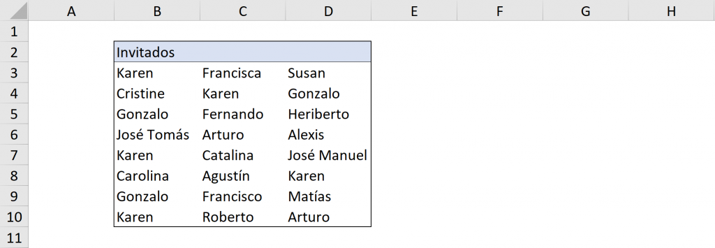
When working with long lists in Excel, you often want to remove or, at least, identify those values that are duplicates and it is very difficult to do it by hand. Finding and removing duplicates is very useful, especially when you are working with lists or databases that contain a lot of information. Using conditional formatting and the “Data” tab you will be able to easily find and remove duplicates from your Excel spreadsheets.

The Basics of Finding Duplicates

Concept: Excel considers as a duplicate value those values that appear more than once, that is, it is not only that a value appears only twice, but that it can appear two, three or more times.

Purpose: Identify which cells or set of cells are duplicated in an Excel list. Sometimes you want to eliminate duplicates or simply identify them to do something with that repeated data.

Find duplicates

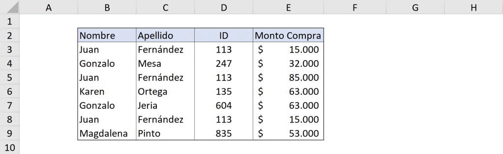
If you have a list of data and want to find duplicates in Excel, you can do it in 3 simple steps. Let's start with the following:

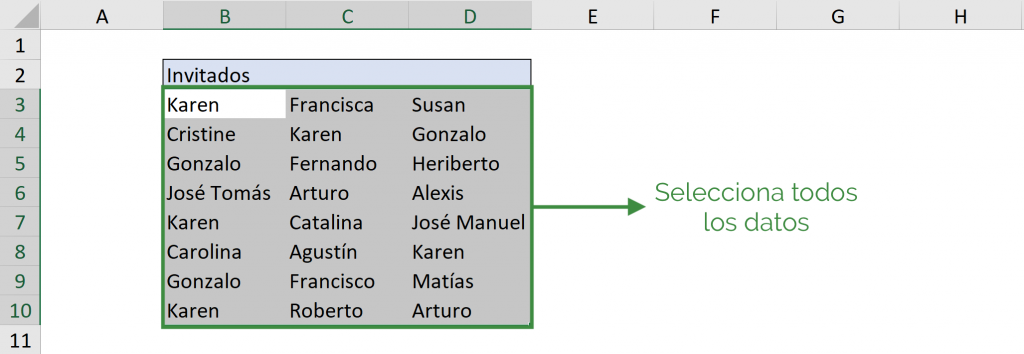
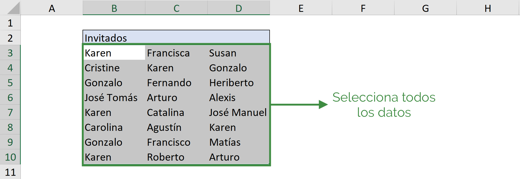
Step 1: Select the data in which you want to find duplicate values.

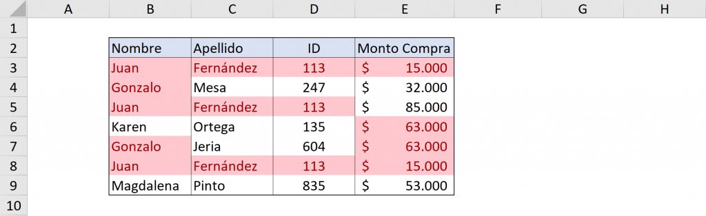
Step 2: In the “Home” tab, select “Conditional formatting”, then “Cell highlighting rule” and finally “Duplicate values…”.

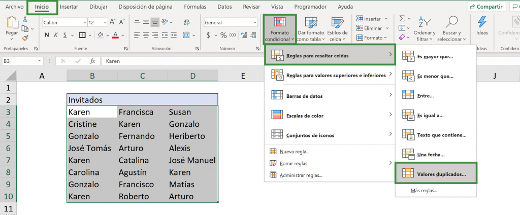Step 3: In the window that opens you can see that it offers you to mark the “Duplicates” and you can also choose the format you want to give to these duplicates. In this case we will choose a light red fill with dark letters. Then, click “Accept”.

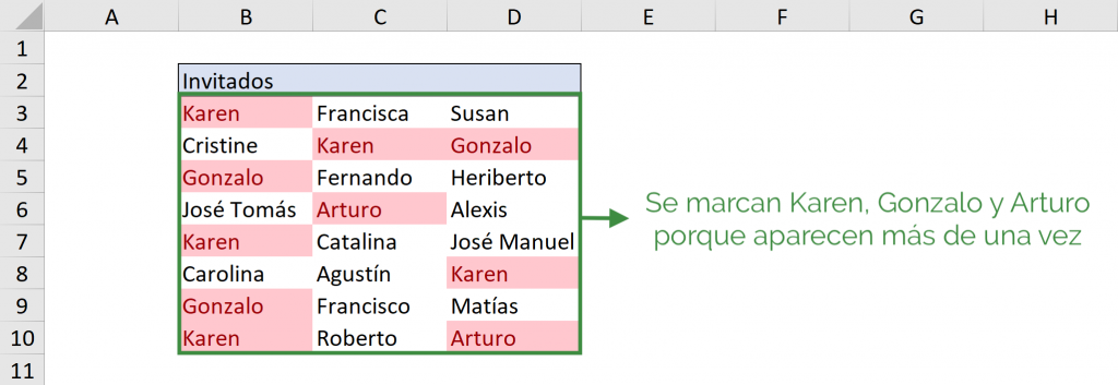
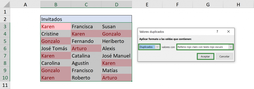As a result, we obtain all duplicate cells in red (remember that in Excel this is the same as repeated), both those that are there twice (Arturo), three times (Gonzalo) or more times (Karen).

To remove the formatting that we just gave to this set of cells, you must go to “Conditional Formatting” and then “Delete rules”.

If you want, you can watch the following video explaining this process with another example:

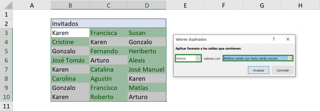
Ninja Tip: To find the unique values you can choose the “Unique” option in the window that opens in Step 3, as seen in the following image:

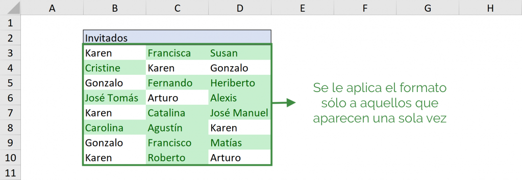
And you get:

Ninja Tip: When evaluating whether a cell is duplicated, Excel takes spaces into account. This means that “Juan”, “Juan·“ and “·Juan” take them as different values. A good option to ensure that these problems do not occur is to use the SPACES function, which leaves only one space between two words and eliminates spaces at the ends of sentences.

Find duplicate value a defined number of times

What happens when you want to highlight those values that are only there three times (not twice, not four or more)? For this you must create a new rule. These are the steps to follow.

Step 1: Select the data in which you want to find duplicate values.

Step 2: In the “Home” tab, select “Conditional Formatting” -> New Rule

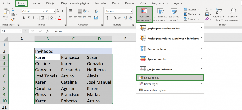
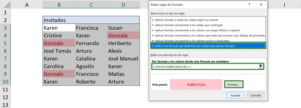
Step 3: In the window that opens, choose the option “Use a formula that determines the cells to format” and write the following formula: =COUNTIF($B$3:$D$10;B3)=3

Step 4: Then, you can choose the format you want to give the triplicates. In this case we will choose light red filling with dark letters. Finally, click “Accept”.

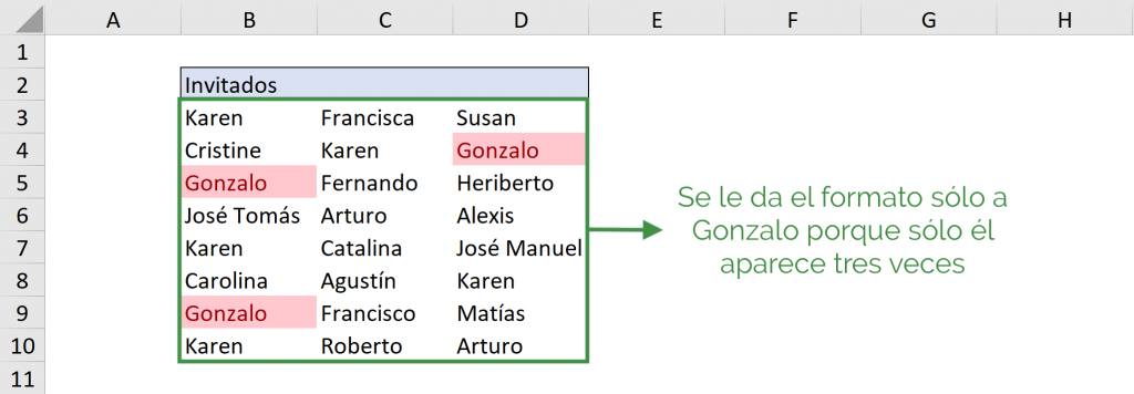
As a result we obtain in red only the cells repeated three times (Gonzalo):

How does =COUNTIF($B$3:$D$10;B3)=3: work?

The formula is used COUNT YES to count the number of cells in the range from B3 to D10 that are equal to cell B3 and if that number is equal to 3, then it formats the cell as red. In this case, it will count how many times “Karen” is there from B3 to D10. Then, since Karen appears 4 times, it is not assigned the red format (because it is only shown if it is there 3 times).

As in Step 1 we selected all the data before going to “Conditional formatting”, Excel automatically copies the formula for all the cells in the selection, but using relative references. So in the cell B4 has the formula: =COUNTIF($B$3$D$10;B4)=3 and thus each cell uses the same formula but comparing the value of the other cells with its own value. In this case, Excel will count how many times “Cristine” appears from B3 to D10. Since it only appears once, it is not assigned the red format.

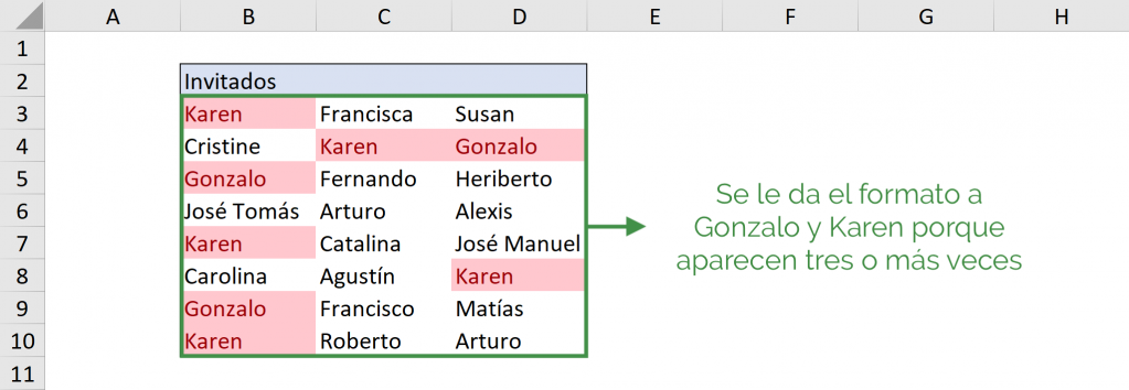
Ninja Tip: You can use any formula you want for this. For example, you can use the formula: =COUNTIF($B$3:$D$10;B3)>=3. In this case, we tell Excel to count duplicates that are repeated three or more times, by using “>=3” (greater than or equal to three) in the expression.

Find duplicate rows

To find duplicate entire rows in your Excel list we can use the method learned above, but the result is not very easy to handle. For example, if we start with the following:

If we apply the newly learned technique we will obtain:

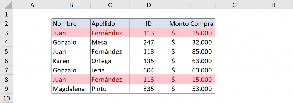
This result is correct but it looks very cumbersome and is not so easy to interpret. We see that Gonzalo is in red but they are two different Gonzalos (one with the last name Mesa and another with the last name Jeria). Also, we see that Juan Fernández has a repeated purchase of $15,000 but another of $85,000, but his name, surname and ID are in red.

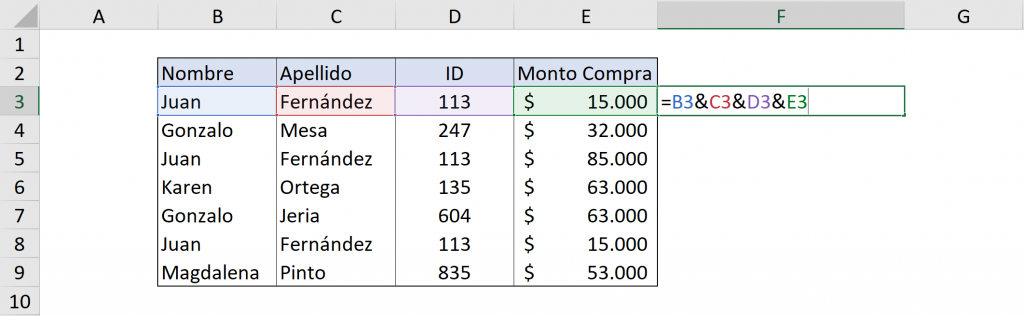
Ideally, what we want is to have the cells in a different format in the case where all the row is duplicated. For this, we will create a new column that is all the values of the row together. You can type in F3: =B3&C3&D3&E3 and then drag down. You can also use the function CONCAT, writing “=CONCAT(B3:E3)”.

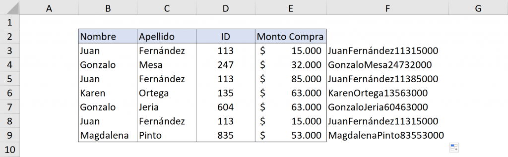Then, we apply conditional formatting to find duplicates on the new column and obtain:

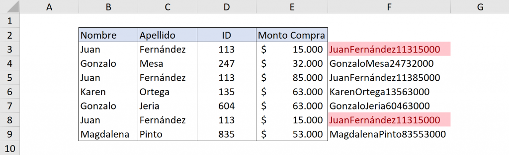
Thus, we have identified the rows that are duplicates in your Excel list. This is because column F is the combination of all the other columns, so by seeing if column F has duplicates we are seeing if there is a duplicate that is identical in all the columns.

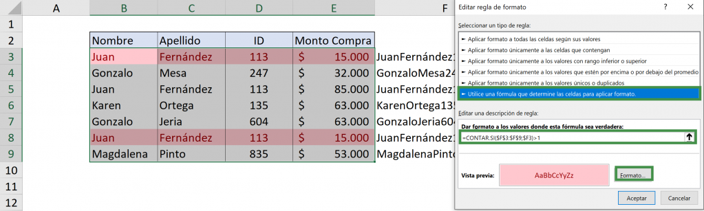
That may be enough, but we had said that we were going to format the entire row, not an extra column. For this you must follow steps similar to the previous item:

Step 1: Select the data in which you want to find duplicate values.

Step 2: In the “Home” tab, select “Conditional Formatting” -> New Rule.

Step 3: In the window that opens, choose the “Classic” Style and the option “Use a formula that determines the cells to apply formatting.”

Step 4: Write the following formula: =COUNTIF($F$3:$F$9;$F3)>1

Step 5: Next, you can choose the format you want to give to the duplicate rows. In this case we will choose light red filling with dark letters. Finally, click “Accept”.

Thus, we obtain:

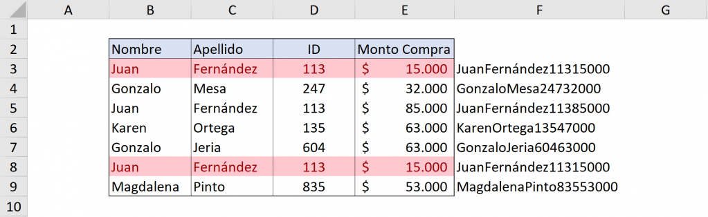
As for =COUNTIF($F$3:$F$9;$F3)>1, it is a similar procedure to the previous section. In this case, we want to compare the value of a cell in the new column with the rest of the column. Thus, for cell B3 the criterion for formatting it red is to count the number of times the value of F3 is repeated between F3 and F9. We see that the same value is in F8, that gives us a result of 2. That is greater than 1, therefore it is given a red format.

Then, for C3 the same thing will happen: the red format will be assigned depending on the number of times F3 appears between F3 and F9, so it is also formatted. Thus, the mechanism is repeated for the entire row and it remains in the red format.

Then, for B4 the criterion is whether the value of F4 is repeated between F3 and F9. Since it is not repeated, it remains with its original format and that is how it is for that entire row. Thus, all the data is traversed and only the duplicate rows remain with the red format.

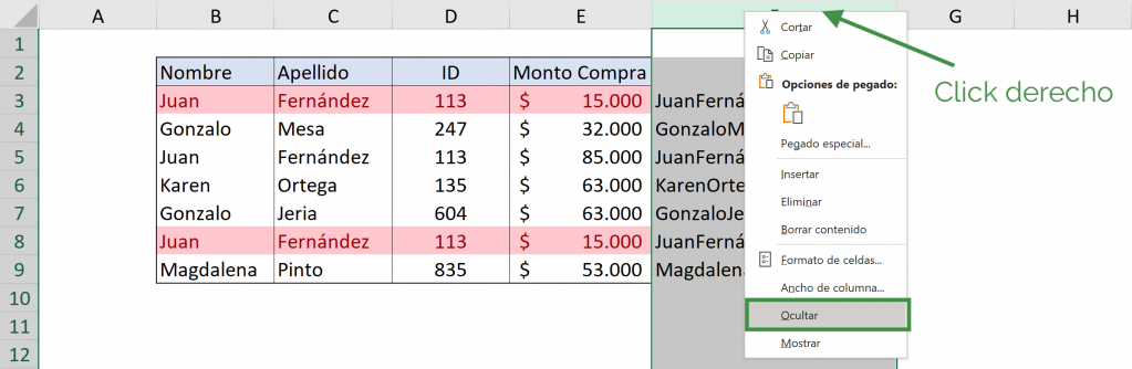
Ninja Tip: If you do not want column F to be seen in which you have everything concatenated, then you can hide it by selecting the entire column and clicking on “Hide”.

And you get:

Remove duplicates

If what you are looking for is to find and remove duplicates, you must follow the following steps:

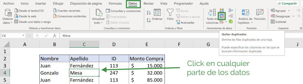
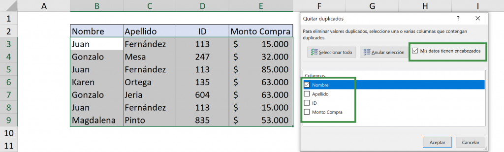
Step 1: Click anywhere in the list or table where you have your data.

Step 2: Go to the “Data” tab and click “Remove Duplicates”.

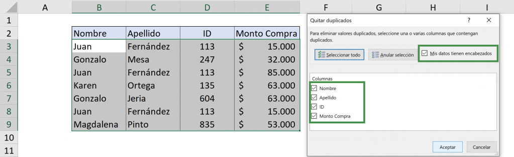
Step 3: In the window that opens, if your list or table has a header (title), check the “My list has headers” option.

Step 4: You must select the columns that will define the criteria for whether the data is duplicated. In this case we will select all because we want to delete the row only if it is 100% repeated. Click “Accept”.

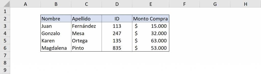
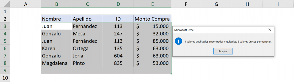And we have as a final result the table in which the purchase of Juan Fernández for $15,000 is eliminated:

Ninja Tip: By finding and removing duplicates you are altering your data, so it is recommended that you have a copy of your original data.

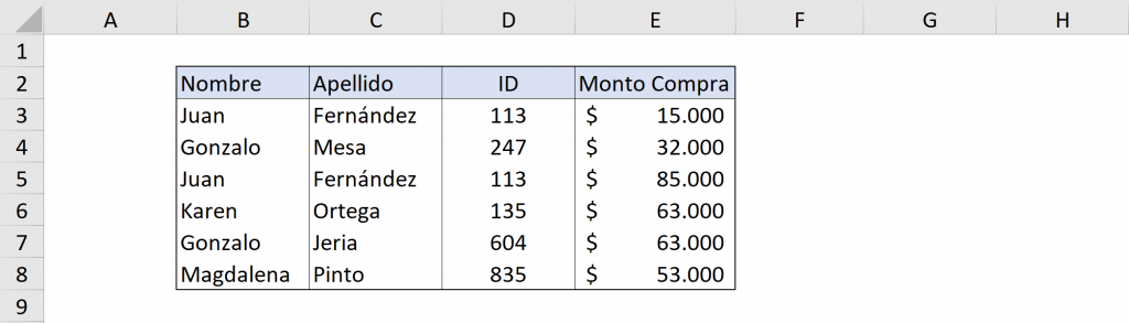
If we wanted, for example, to eliminate all the cells in which “Name” is duplicated, in Step 3 we would select only the “Name” option, as seen in the following photo:

When removing duplicates, the first mention is always kept and the rows below will be removed. Thus, for the name “Juan” only the first purchase by Juan Fernández remains for $15,000 and with respect to “Gonzalo” only Gonzalo Mesa remains, eliminating Gonzalo Jeria.