Shade alternating rows 2 ways in record time

1. The Basics of Shading Alternate Rows

What is shading alternate rows? It is highlighting all the even rows or all the odd rows in a table, in an interspersed manner.

What is it for? It serves to visualize the information better in a table. When we have a large amount of data, it is useful to distinguish the information that each of the rows gives us. Avoid confusion between them.

Clearly shading rows can be done manually, but it would take a long time! Therefore, we teach you ways to do it quickly.

To shade alternate rows there are two methods: using conditional formatting or using an Excel table style. We will look at both below.

2. Shade alternating rows with conditional formatting

Shade alternate rows with conditional format It consists of creating a rule so that this action is executed through a specific formula. Let's see how to apply it!

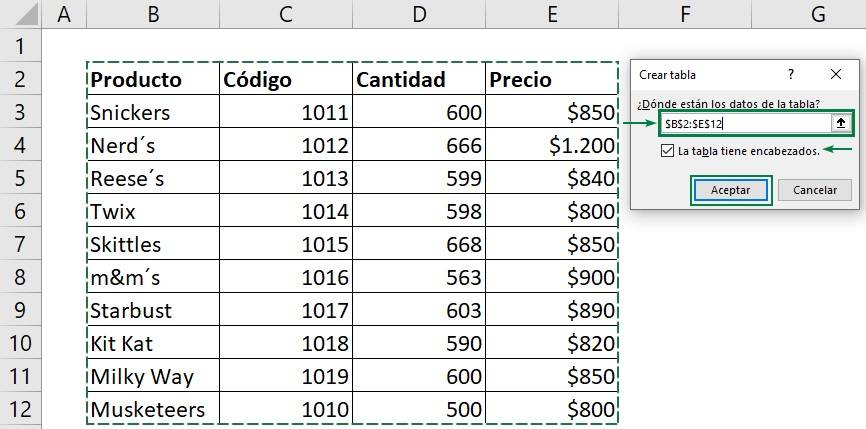
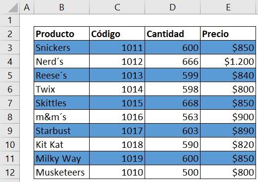
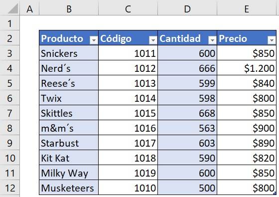
We have the following table with different products sold in a candy store, along with their codes, quantities and prices.

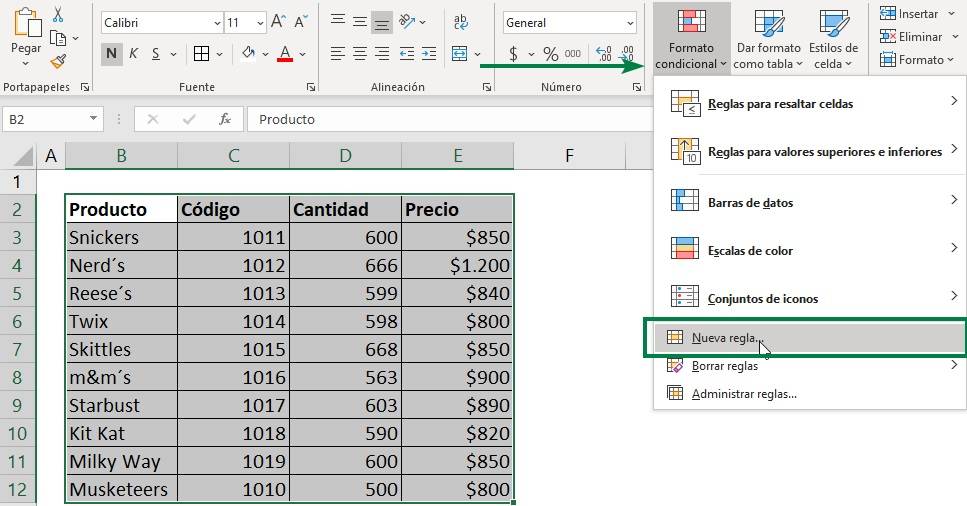
1. First, we select the range of the table where we want to shade the interleaved rows. In “Home”, in “Styles”, we go to “Conditional formatting”, and press “New rule”, as shown below.

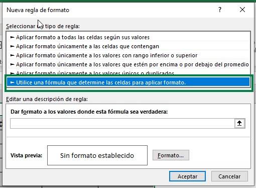
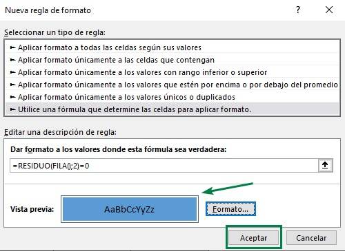
2. The following box appears, where we put the option “Use a formula that determines the cells to apply the format”.

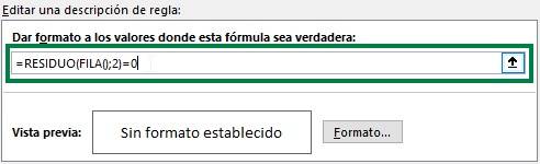
3. Then, in the space indicated, we write the formula RESIDUE(ROW(); 2) = 0 to shade alternating rows, as the image below shows.

What do these formulas mean for shading alternate rows?

The RESIDUE function returns the remainder of a division. The row function indicates the number of each row. In this case, the row number (ROW()) is divided by 2. For example:

• The division of the Snickers row will be 3 divided by 2. In this case the RESIDUE function returns remainder 1.
• For the Nerd's row, however, it will be 4 divided by 2. The RESIDUE function gives us the remainder 0.

Then what we do is set this formula equal to zero, what does it mean?

It means that, if the remainder of the division is zero, it is true, and therefore the indicated format is applied to it. In this case they will be all even rows.

While odd rows, which have a remainder other than zero, will not change their format.

If we want to shade alternate odd rows, we will change the formula and set it equal to one instead of zero.

4. Then we must give it the format we want. To do this, click on “Format”, and you can choose the option you want! In this case, we will want to shade the interleaved rows a specific color. To do this, we go to “Fill”, select the color, in this case light blue, and click “Accept”.

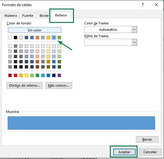
In this way, in the initial box, a preview of the format for shading alternate rows appears, as shown in the image. We click on “Accept”.

And we see our table with the new format! That's how fast it is to shade alternate rows.

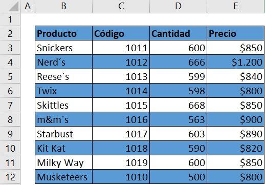
This way we can easily see that the Kit Kat code is 1018, with a quantity of 590 and a price of $ 820. This way we don't get confused with the information from the other lines of Starbust or Vía Láctea.

How do we do it if we want to shade odd, instead of even, alternating rows?

We write now, RESIDUE(ROW(); 2) = 1 , as the image shows. In this way, the divisions with remainder 1 (odd rows) will be the green ones and, therefore, the shaded ones.  

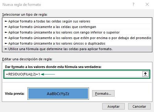
We click “OK,” and see how our table changes to shade alternate rows! Now the line for Snickers, Reese's, Skittles, Starbust and Milky Way are shaded, when they weren't before.

3. Shade rows iinterspersed with excel table style

We can shade alternate rows using the predefined tables that Excel provides us.

How do we apply this option?

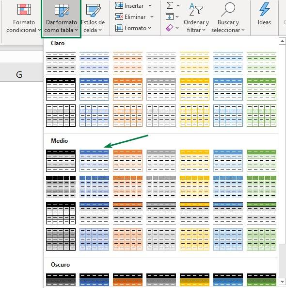
1. In “Home”, we go to “Styles” and click on “Format as table”. Highlight alternatives other than “Light”, “Medium” or “Dark”. In this case we select a “Medium” option to shade alternate rows, as shown in the image.

2. The following box appears where we must select the range of the table where we want to shade alternate rows. We select, click on “The table has headers” and “OK”.

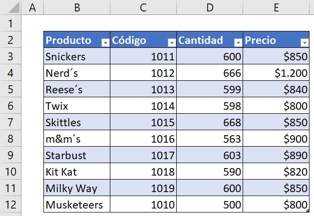
The table looks like this, with interspersed rows of light blue, it's that simple to shade alternate rows with Excel tables!

• How do we shade alternate columns instead of filas?

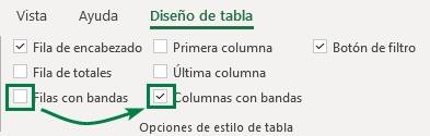
We go to “Table Layout” and we go to “Table Style Options”. There we can modify the table according to how we want, such as inserting a row of totals, removing the filter button, etc.

To shade columns, we must deactivate the “Banded Rows” option, and apply the “Banded Columns” option, as the image shows.

This is how we see how our table changes, now with alternating shaded columns!

• ¿ But What happens if we don't want a table with its properties and we only want to have a range of cells? How do we do it?

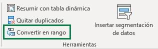
We select any cell belonging to the table, go to “Table Design”, in “Tools” and click on “Convert to range”.

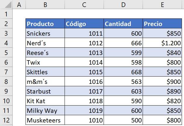
This will leave us with a normal range of cells, as shown in the image, without table formatting and similar to method 1 of shading interspersed rows with conditional formatting.

With these two methods we have seen how to shade alternate rows quickly, What are you waiting for to apply them and better visualize your data? Apply what you have learned and you will see how useful it is when working with databases.

Frequent questions