Conditional formatting: Highlight values quickly

What is conditional formatting in Excel?

He CONDITIONAL FORMAT is an Excel tool that allows you to automatically apply a certain format to those cells that meet certain requirements. This allows you to find and highlight values more quickly and visually.   

What is conditional formatting for?

• Purpose: Conditional formatting changes the appearance of cells based on whether they meet a condition. If the condition is not met, the cell will maintain the original format. 
• Characteristics: Rules that are created for conditional formatting can be cell value-based or formula-based rules.
• Advantages: Facilitates the process of highlighting cells or analyzing data visually. In addition, it allows you to find the values you are looking for quickly.

This tool can be used on any type of data matrix, even pivot tables

Tip Ninja: If you want to know more about pivot tables, we recommend you visit this article.

Another common use of conditional formatting is to highlight alternating rows. If you want to learn how to do it, we recommend visiting this Blog.

How to apply conditional formatting in Excel?

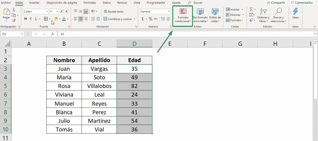
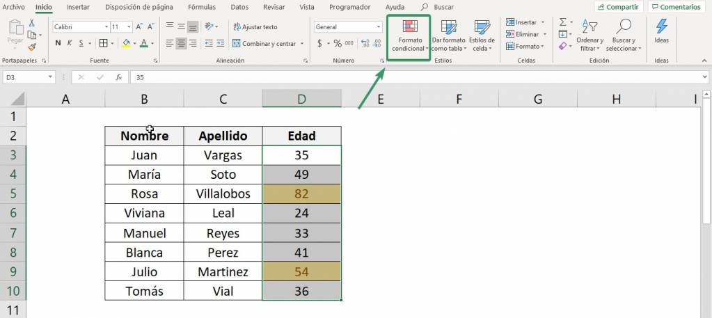
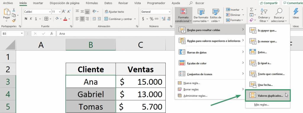
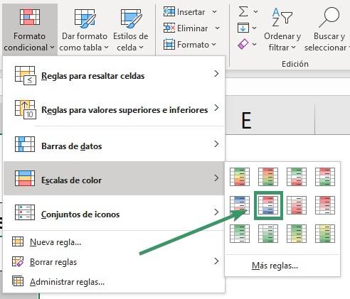
To apply conditional formatting to certain data, the first thing you must do is select the data and then, on the Home tab, within the Styles group, select the “Conditional formatting” button, as shown in the following image.

Then you choose the type of conditional formatting you want and that's it!

Types of conditional formats

There are different types of conditional formats in Excel, in this article you will learn how to use the six most common ones.  

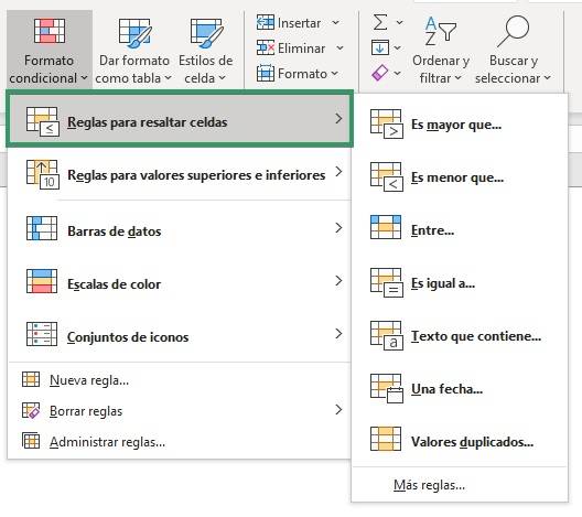
Rules for highlighting cells

Using the Conditional Formatting “Cell Highlighting Rules” tool, you can highlight cells that meet certain requirements, such as the following:

• Is greater/less than: Highlights those cells with values greater/less than the determined one.
• Between: Highlights those cells whose value is between two specific values.
• Is equal to: Highlights those cells that contain the same value as the determined one.
• Text containing: Highlights those cells that contain the same given text. 
• A date: Highlights those cells that correspond to the given date, for example, yesterday.
• Duplicate values: Will highlight those cells that have identical values.

From each of these conditional formatting modes you can choose the format you want, such as font color, cell background, borders, among others.

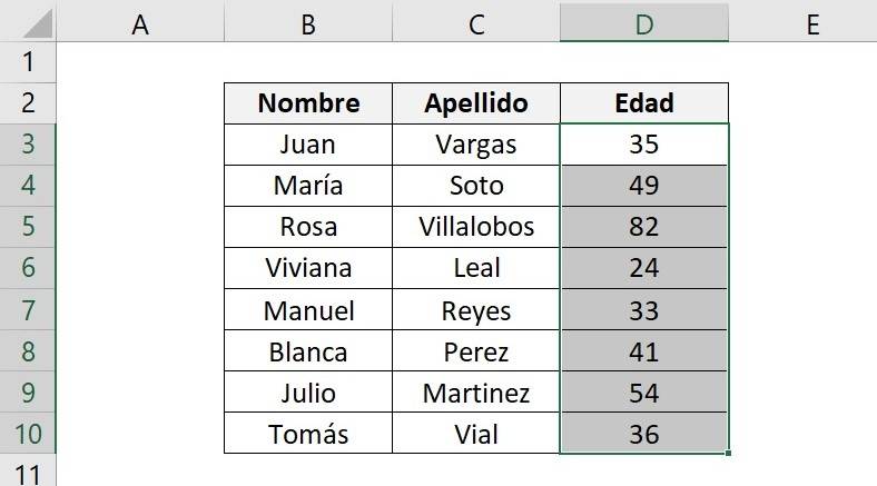
To understand how this type of Excel conditional formatting works, let's look at a simple example. Let's consider the following list of people with their respective ages. Suppose we want to highlight in yellow those ages over 50 years old.

1. Select the range of cells that contains the ages.

2. In the “Home” tab, click on “Conditional formatting”

3. As we are looking to highlight certain cells, click on “Rules for highlighting cells”. A new menu of options will open, but since we are looking for ages over 50, we must click on “Is older than…”

4. A dialog box called “Is greater than” will open. In it we must write the determined requirement, in this case, since the age must be greater than 50, we must write the number “50”. It also gives us the option to choose the type of format, in our case, we want it to stand out in yellow, therefore, we choose the second option.

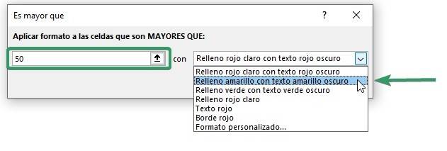
5. Click “Accept”.

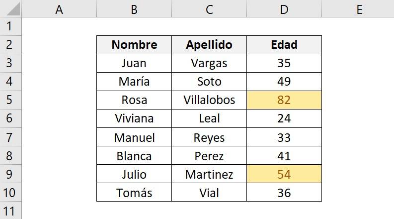
We can see that the conditional formatting highlighted in yellow only those cells that contain an age greater than 50. 

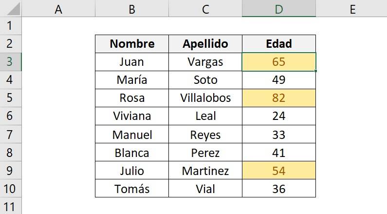
6. If an age value changes, Excel Conditional Formatting will check to see if it is greater than 50, and if it is, it will automatically highlight that cell. For example, if we change Juan Vargas' age to 65, we can see that he will be highlighted in yellow.

Upper and lower rules

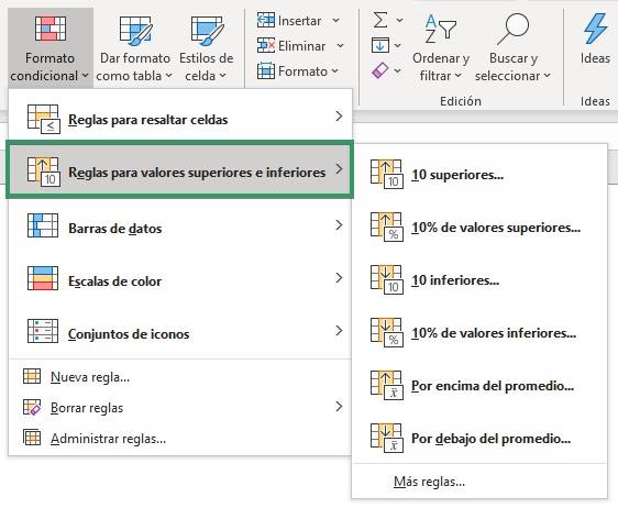
Using the “Rules for higher or lower values” tool in conditional formatting, you can highlight cells that meet certain requirements, such as the following:

• top 10: Highlights those cells that contain the 10 values with the highest value within the cell range. In addition, it gives the option to change the number 10 for any other.
• 10% of higher values: The 10% of the total cells containing the largest values will be highlighted.
• bottom 10: Highlights those cells that contain the 10 values with the lowest value within the cell range. In addition, it gives the option to change the number 10 for any other.
• 10% lower values: The 10% of the total cells that contain the smallest values will stand out.
• Above average: It will highlight those cells that are greater than the average of the selected cells.
• Below average: It will highlight those cells that are less than the average of the selected cells.

Continuing with the example, now we want to know those ages that are above the average age.

1. Select the range of cells that contains the ages.

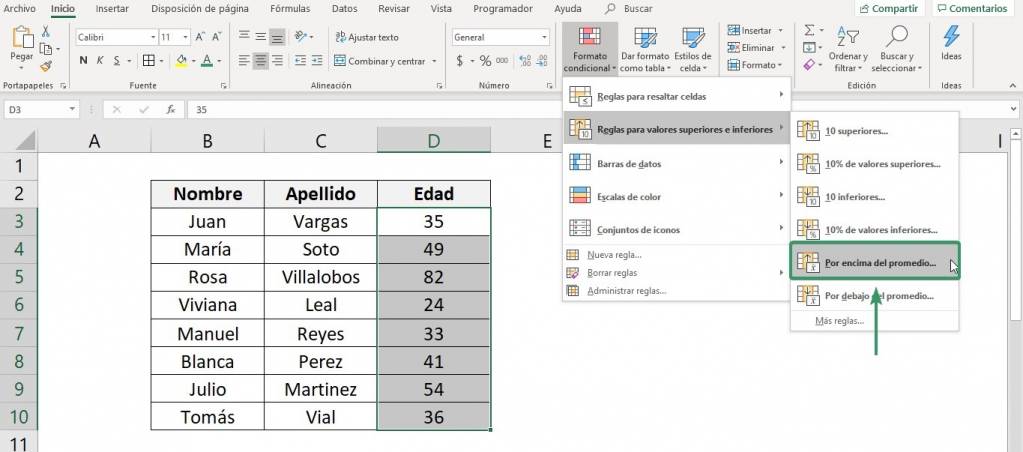
1. In the “Home” tab, click on “Conditional formatting”, then click on “Rules for upper or lower values”. A new menu of options will open, but since we are looking for those ages above average we must click on “Above average…”

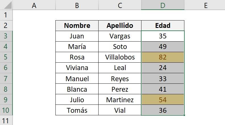
2. A dialog box called “Above average” will open, in which we must choose the type of format, in our case, we want it to stand out in red, therefore, we choose the first option.

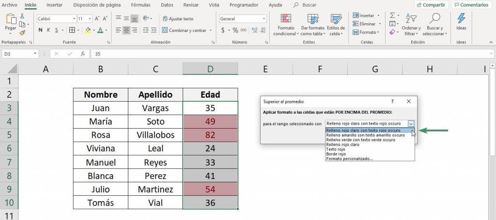
3. Click “Accept”

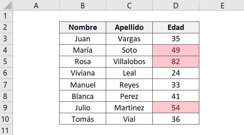
We can see that the conditional formatting highlighted in red only those ages that are above the average.    

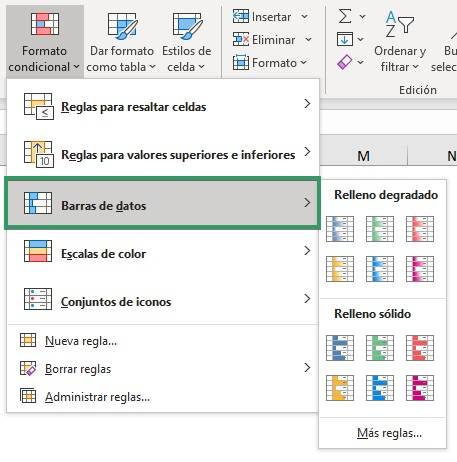
data bars

This type of conditional formatting allows you to create a small graph for each value which makes it easier to compare values. Each value is represented in a new cell, where its length will depend on the corresponding value and will be relative to the rest of the values.   

To better understand this type of conditional formatting, let's apply it to our ages example. We want to see how the ages of each person look graphically in comparison to the other ages.

1. Select the range of cells that contains the ages.
2. On the “Home” tab, click “Conditional Formatting,” then click “Data Bars.” A new menu of options will open with different colors to choose from, we will choose the gradient light blue.
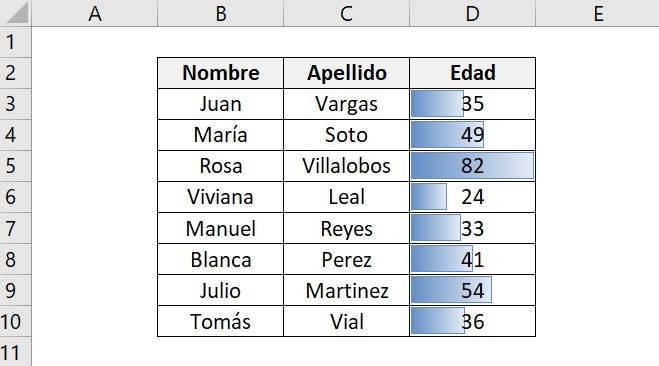
3. Ready! We can see that the highest value, that is, Rosa's age, is the one with the longest bar and from this value the bars will have a smaller size.

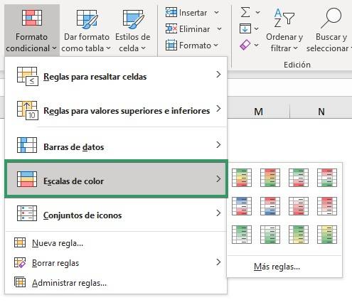
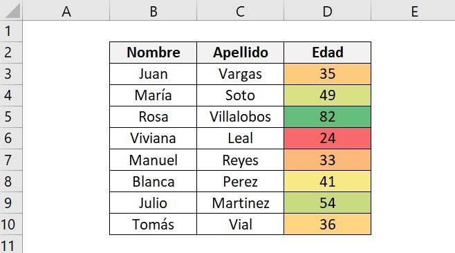
color scales

This type of conditional formatting allows you to modify the background of a cell according to its proximity to the maximum and minimum values within the selected data range. The tone of each cell will depend on the proximity to either of these two extremes. 

To better understand this type of conditional formatting, let's apply it to our ages example.

1. Select the range of cells that contains the ages.
2. On the “Home” tab, click “Conditional Formatting,” then click “Color Scales.” A new menu of options will open with different colors to choose from, we will choose the first option which consists of tones between green and red.
3. Ready! We can see that the highest value, Rosa, is the one with the green bar and the lowest, Viviana, the red bar. The other ages vary their tones depending on how close they are to these values.

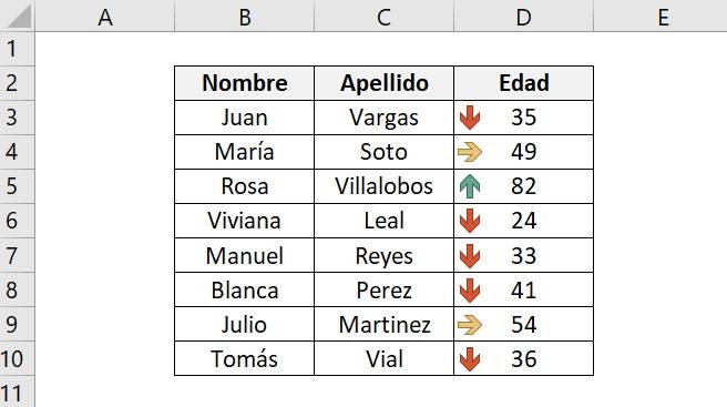
Icon Sets

Icon set conditional formatting allows you to mark those cells with the icons you want depending on the values of the data set we have.

Let's apply this format to our example to understand better.

1. Select the range of cells that contains the ages.
2. On the “Home” tab, click “Conditional Formatting,” then click “Icon Set.” A new menu of options will open with different colors and shapes to choose from, we will choose the first option which consists of the set of three arrows.
3. Ready! We can see that the arrows vary their color depending on how high the age value is. Rosa's age, which is the oldest, has a green arrow, however, the youngest, Viviana, has a red arrow. 

Conditional formatting with formulas

Another way to use Excel's conditional formatting is to apply a formula, where Excel will highlight those cells that meet the given formula. We must know that formulas in conditional format must evaluate to TRUE or FALSE.

Now, we want to know those ages that are odd. For this, we must use the IS.ODD function, this function returns TRUE if the number is odd and FALSE if it is even. 

1. Select the range of cells that contains the ages.

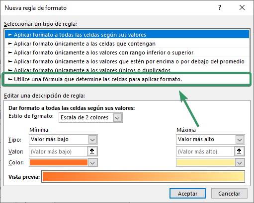
2. In the “Home” tab, click on “Conditional formatting”, then click on “New rule”

3. A dialog box called “New formatting rule” will open within the list of options, we must select “Use a formula that determines the cells to apply formatting.”

4. In the lower box we must insert the function, in this case, IS.ODD.

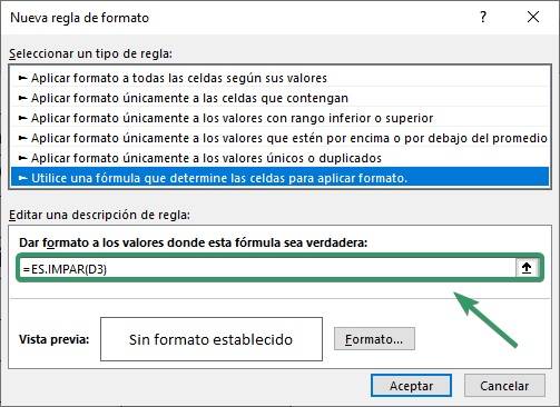
That is, the IS.ODD function is as follows:

Tip Ninja: In the formula you should always write the upper left cell of the selected range. Conditional formatting will copy this formula to the other selected cells.

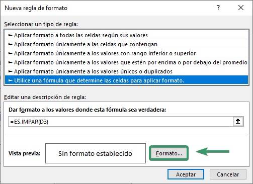
5. Click on the “Format…” button

6. A new dialog box called “Format Cells” will open, here you can choose the color with which the cells will stand out, the type of border, the font, among others. We choose a light blue fill color.

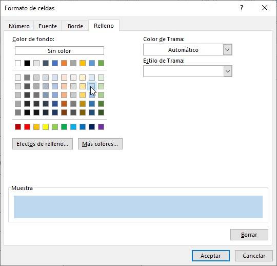
7. Click “OK” in both dialog boxes.

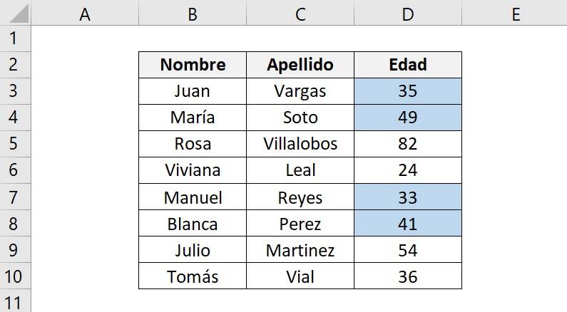
We can see that the conditional formatting with formula highlighted only those cells with odd ages in light blue. 

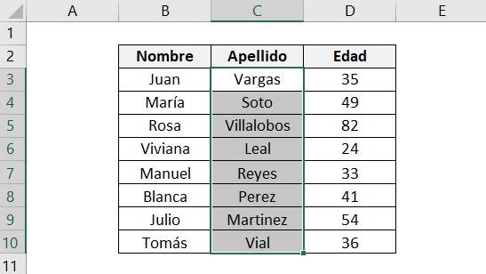
Let's look at another example. Now, we want to know those people with the last name “Soto”, for this, we must use a formula that tells the conditional format to search in the last name cells, those that contain the word “Soto”.

1. Select the cells that contain the last names.

2. As in the previous example, click on “Conditional formatting”, then “New rule”. In the dialog box called “New Formatting Rule” within the list of options, click “Use a formula that determines which cells to format.” In the lower box we must write the formula.

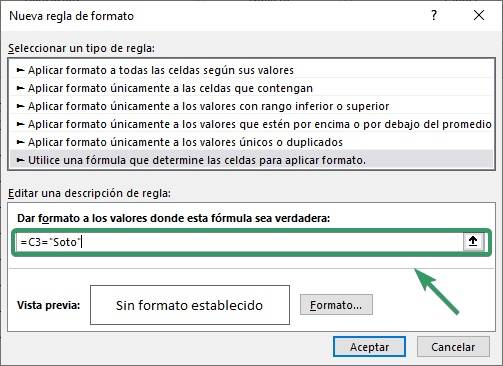
That is, the formula is the following:

The formula will tell the rule to highlight those cells that are equal to the word “Soto”

Tip Ninja: Remember that, when searching for a text value, we must write it in quotes, otherwise Excel will not recognize it.

3. We choose a format for the highlight. In this case, we choose the color green.

4. We click on “Accept”.

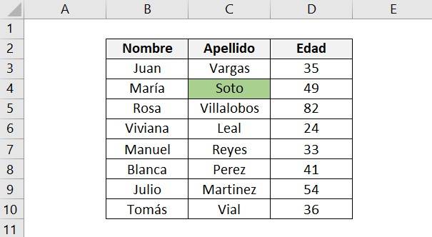
We can see that the conditional formatting highlighted in green those cells that contain the word “Soto”, in this case, only one person has the last name Soto.

Tip Ninja: If the formula used returns an error in a cell, we recommend using the IFERROR function or the IFND function. These functions allow you to control errors.

If you want to learn more about this Excel tool, we recommend you watch the following video. In it you can learn more ways to use conditional formatting.

Clear conditional formatting rules

To delete used conditional formatting rules, Excel allows you to delete only some or all of the conditional formatting rules on the sheet.

1. Select the range of cells that contains the conditional formatting rule, in this case, the ages.

2. In the “Home” tab select “Conditional formatting”

3. Click on “Delete rules”. A new menu of options will open, but since we want to delete the rule that we put on the ages, we must click on “Delete rules from selected cells”

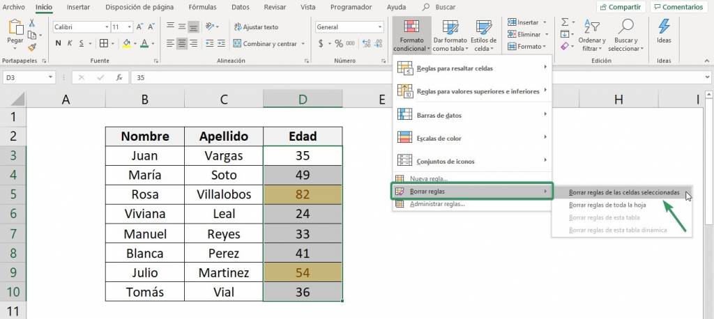
Tip Ninja: If you have many conditional formatting rules, we recommend clicking on “Delete rules from the entire sheet”, this way all the rules will be deleted automatically.

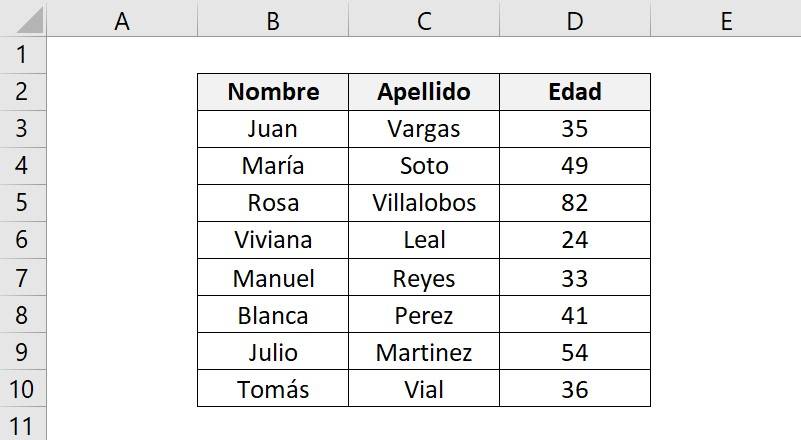
4. We can see that no cell in our data table is highlighted.

Examples of conditional formats

Highlight duplicate cells with color

Excel's conditional formatting also allows us to highlight duplicates in our data. This option works for all types of data, whether numbers, texts, dates, among others. 

Let's look at an example where we have the amount sold to each client within a month. We would like to know who are the customers who buy more than once a month. To highlight duplicate values, follow these steps:

1. Select the data you want to analyze.

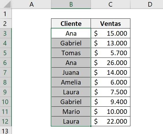
2. On the “Home” tab, click “Conditional Formatting,” then click “Highlight Cell Rules.” A new menu of options will open and click on “Duplicate Values”.

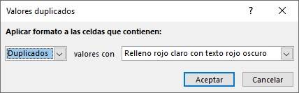
3. A “Duplicate Values” text box will open, choose the format you want and click OK.

4. Ready! We see that some cells were highlighted in red because they have a value that is repeated at least once. Cells that are not highlighted are because they contain a value that is not repeated. 

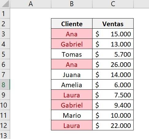
We can see that those customers who buy more than once are Ana, Gabriel and Laura.

Example 2

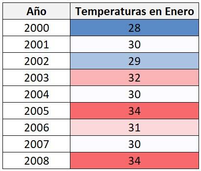
Suppose we have the maximum temperature for the month of January in different years and we want to analyze whether the temperature has been increasing or decreasing year by year.

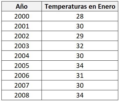
For this we can use various types of conditional formatting, but to see it visually, we will use the color scale format. 

1. We select the maximum temperatures in January.
2. Then we click on “Conditional formatting”, then on “Color scales”
3. We generally represent high temperatures with the color red and low temperatures with blue, which is why we choose the color scale that contains those colors. It is important to know that the color that appears above will be associated with the highest numbers and the one below with the lowest values, for this reason, we choose the scale that begins in red and ends in blue. 

4. Ready! We can see that, although the temperature increases and decreases over the years, there is a certain increase in temperature.

Example 3

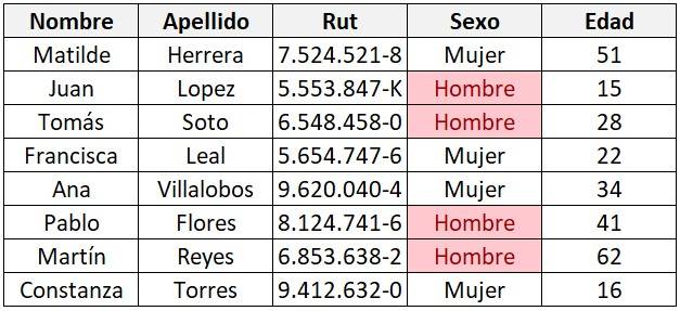
Suppose we have a database with the personal data of different people and we need to know who are men and over 20 years old.

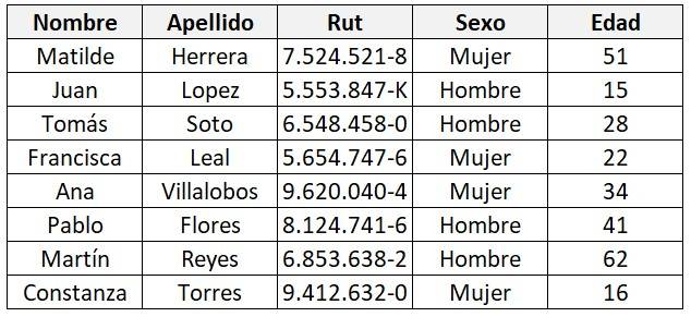We can see that we must make two conditional formats, one for sex and another for age.

Let's start with the format for sex. For this we can use “Rules to highlight cells” and use the “Equals” format. 

1. We select the sex data range and within Rules to highlight cells we click on “Equals”.
2. In the text box we must say that we want to highlight those cells that are equal to “Man”, therefore, we write =”Man”.

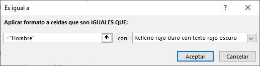
3. We click on Accept and that's it, we already have those male people highlighted in red.

Now, to identify people older than 20 years old, we can use the “Rules for highlighting cells” format type and use the “Is older than” format.

1. We select the age data range and within Rules to highlight cells we click on “Is older than”.
2. In the text box we must say that we want to highlight those cells that are greater than 20, therefore, we write 20.   

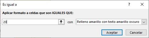
3. We click on Accept and that's it, we already have those people who are over 20 years old highlighted in yellow.

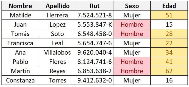Now we can see who are men and are over 20 years old since they must have both cells highlighted, therefore, we know that Tomás, Pablo and Martín meet both requirements. 

Conclusions

Excel conditional formatting is a very useful tool as it serves to highlight data that meets specific conditions by applying a selected format such as color, size, font, among others. In addition, it allows you to quickly and visually identify duplicate data. 

Frequent questions

When to use conditional formatting in Excel?

Conditional formatting in Excel is useful when we need to analyze certain values as it allows you to highlight cells that meet certain criteria. For example, for a company it may be necessary to highlight in red those accounts with a negative balance in order to quickly identify losses. 

What are the advantages of using conditional formatting?

Excel's conditional formatting makes it easy to highlight cells or analyze data visually. In this way, it allows you to find the values you are looking for quickly. Additionally, this tool can be used on any type of data matrix, even pivot tables.

Frequent questions