FUNCTION O: Master it in 4 simple steps.

Key information

The function EITHER is an Excel logical test that returns values of true or false depending on whether two EITHER more conditions. It is especially useful to combine with other Excel tools, such as the function YEAH. 

The basics

• Purpose- The OR function allows you to check whether a cell or set of cells meets one or more conditions. 
• Characteristics: Cells can be considered individually or as a range to define where the established condition must be met. 
• Syntax: =O(logical_value1; [logical_value2]; [logical_value3]…)
• Arguments:
  • logical value = cell or set of cells for which a condition to be met is defined. 
• Result: True or false. The function returns TRUE when any of the established logical values is met. The function returns FALSE when none of the logical values is fulfilled. 

OR function with a condition

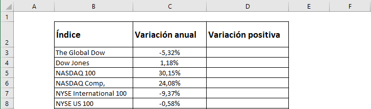
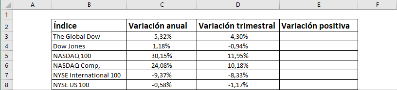
Consider the following table that contains information on stock market indices and their annual percentage variation. We want the third column to indicate whether the variation has been positive. 

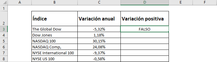
Step 1: Go to the first cell in the “Positive Variation” column. We want the cell to return TRUE if the “Annual variation” column is positive, that is, greater than zero. 

Step 2: Once the formula is written correctly, press Enter. We see that the result is FALSE since the value we are considering is not greater than zero. 

Step 3: Position yourself in the lower right corner of the cell where you wrote the formula, until your mouse turns into a black cross. 

Ninja Tip: You can skip this step by selecting the cells where you want to drag the formula, and then press Ctrl + J if you have Windows or Ctrl + D if you have Mac. With this shortcut you achieve the same result using only the keyboard. You can learn more about shortcuts in Excel in this post. 

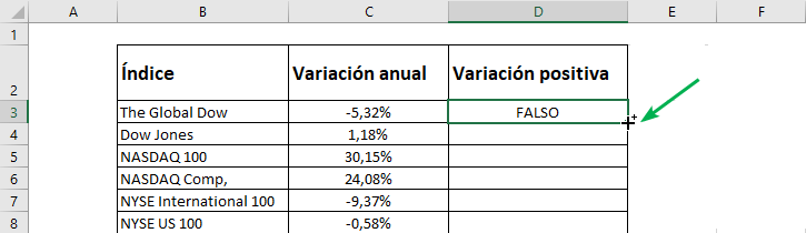
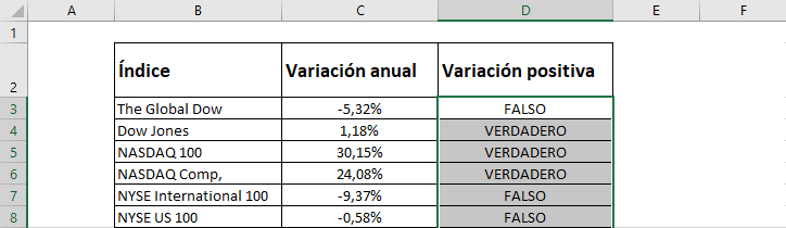
Step 4: Double click to drag the formula. That's it! We see that when the values are positive, the formula returns TRUE. Otherwise, it returns FALSE. 

OR function with more than one condition

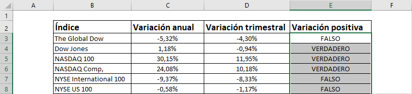
Now consider that the table contains an additional column with the quarterly variation. Now we will look for the function to return TRUE if the annual variation or the quarterly variation is positive. 

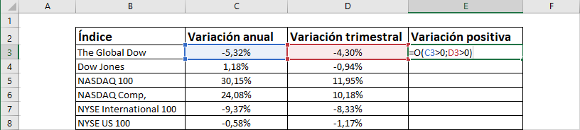
Step 1: Go to the first cell in the “Positive Variation” column. We want the cell to return TRUE if the column “Annual variation” or the “Quarterly variation” is positive, that is, each one greater than zero. 

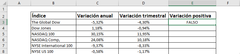
Step 2: Once the formula is written correctly, press Enter. We see that the result is FALSE since both the value of “Annual variation” and “Quarterly variation” are negative. 

Step 3: Position yourself in the lower right corner of the cell where you wrote the formula, until your mouse turns into a black cross.

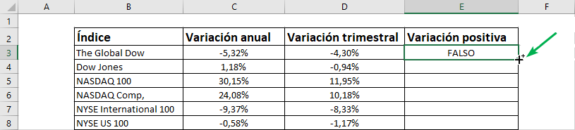
Step 4: Double click to drag the formula. That's it! Note that it always comes out TRUE when either “Annual change” or “Quarterly change” are positive (like “Dow Jones”), and FALSE when both values are negative (like “The Global Dow”). 

Ninja Tip: You can also use the function with words. In that case you can only use the “=” symbol, and remember to put the words in quotes. 

Combining IF and OR function. 

The IF function is a very useful tool that allows you to return different results depending on whether a condition is met. Unlike the OR function, you can only set a single condition, but at the same time you can choose the values you want to be returned depending on whether the condition is met or not, such as “Pass” and “Fail”, “Grade” and “ Doesn't qualify,” or anything else. Considering this, combining both functions allows you to get the best of each to achieve your goal. 

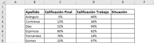
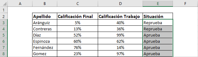
Now suppose the following table contains information about student grades. The course is approved if the final grade is greater than 50% OR if the assignment grade is greater than 80%. Additionally, we would like “Status” to indicate “Pass” or “Fail” depending on whether the condition is met or not. In this case, satisfying the condition will depend on what the OR function returns: if it returns TRUE, then the condition is fulfilled for IF (and vice versa for the opposite case).  

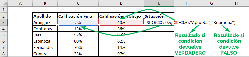
Step 1: Go to the first cell in the “Situation” column. Write the formula starting with the IF function. The first element of the function is the condition, which in this case you must fill with the OR function. The logical values correspond to those we just mentioned above. After finishing writing the OR function, you must choose the values that the IF function will return if it is true or not. In this case, “Approve” or “Fail”. 

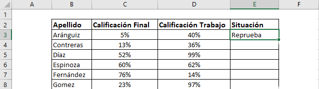
Step 2: Press Enter. We see that the result is “Fail” since Aránguiz did not obtain a grade above 50% in “Final Qualification” or 80% in “Work Qualification”. 

Step 3: Drag the formula down with the mouse or keyboard shortcuts, as indicated in Step 3 and Step 4 in the previous section. That's it! Now we have an IF OR function that fits exactly what you need. 

You already have at least the basic elements to master the O function. As its name indicates, this function is used when you want several conditions to be met but not necessarily together. Now, let's try it!