How to make pivot tables in Excel

Pivot tables in Excel: Synthesize information quickly

What is a pivot table in Excel?

Dynamic tables are tables that group information from a specific database (Excel table), with great capacity to dynamically modify its structure.

What are pivot tables in Excel for?

They help us make different types of analyzes and comparisons through the appropriate combination of information that we insert into our dynamic tables. They are also known by their English name: pivot tables.

You can complement your learning with the following video: 

How to insert a pivot table in Excel?

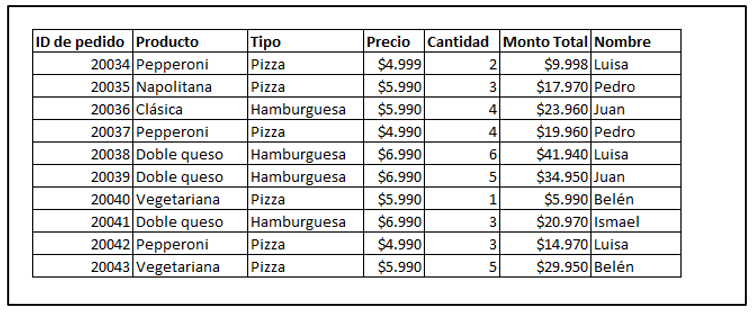
Before we start creating an Excel pivot table, it is important that we have the data in an Excel table organized, as shown in the image below.

How do we start? Excel gives us two options: it recommends dynamic tables for the data we have, or it gives us the possibility of creating our own dynamic table.

Insert recommended pivot table

We go to “Insert”, and click where it says “Recommended pivot tables”.

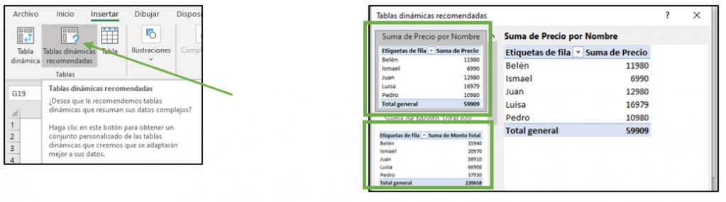Excel will give us different previews to insert our dynamic periodic table. We choose the design that we like the most, and it will appear in a new Excel sheet. Then we will be able to modify this table by changing the fields as appropriate, as we will see below with the option of creating our own ideal table from scratch.

This video shows us how to insert recommended pivot tables:

Create pivot table

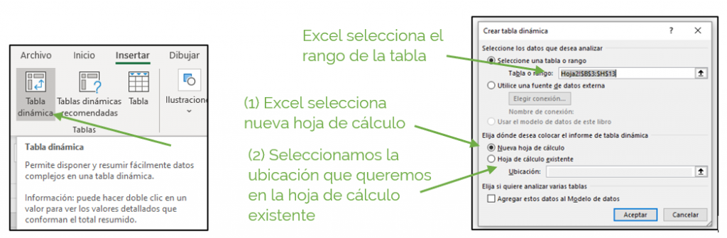
We are going to “Insert” again, but now we are going to the “Pivot Table” option.

The image box appears where Excel automatically selects the range of the table that we want to create, which we could modify if we wanted. Then it gives us the possibility to choose the location of our pivot table:

1. In a new sheet, which is the default option by Excel.
2. In the same spreadsheet, where we must select the place for it.

You can complement this information in the following link ExcelTotal.

In this video you can see how to create dynamic tables:

How to make a pivot table in Excel step by step

How do we design our pivot table?

Next, Excel shows us the “PivotTable Fields”.

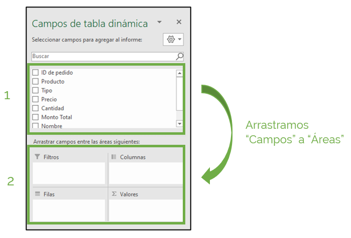
Field List

It corresponds to the first part where all the existing fields or information are listed.

Report filter

It will allow us to select which aspects we want to see in the table.

Column labels

It will allow us to organize our information by columns.

Row labels

It will allow us to organize our information by rows.

Values

It will allow us to view the information inside the dynamic table, for which we must select the type of operation we want, that is, the calculation values: sum, count, average, maximum, minimum, etc. Excel automatically selects the “add” operation, which we can modify later.

This way we can decide what our table will be like, and we can play around iterating different types of pivot tables! In this way, with an appropriate combination of the fields, we can reach the schema we want, and quickly perform correct analyzes using the dynamic tables.

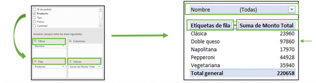
How do we drag the fields?

In our example, we moved “Name” to “Filters”, “Products” to “Rows”, and “Total Amount” to “Values”. And we obtain the following dynamic table, where we can see, for example, that with the “Double cheese” burger we obtain a greater amount.

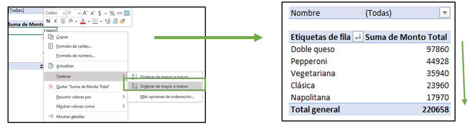
How do we order the fields?

We can order our pivot table according to our own interests to view the dynamic tables in a better way. How do we do it if we want the products to appear from highest to lowest amount? We right click on any cell within the “Sum of Total Amount” column, go to “Sort”, and then we can sort as we wish, in this case from “Highest to lowest”. And our dynamic table looks like the image shows.

How do we configure the fields?

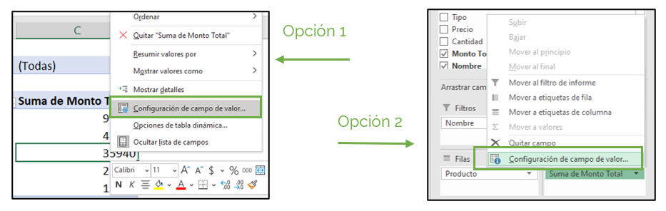
Excel in the “Values” area automatically selects the addition operation, but we can change it to whatever we want depending on the type of information we want to compare, how to do it? We can do it in two ways:

(1) Go to any cell in the “Sum of Total Amount” column, right-click and select “Value Field Settings”.

(2) Or, we go to the box on the right where the fields of our pivot table are, and go to the “Values” area, where we click on “Total Amount Sum”, and then select “Value Field Settings” ”.

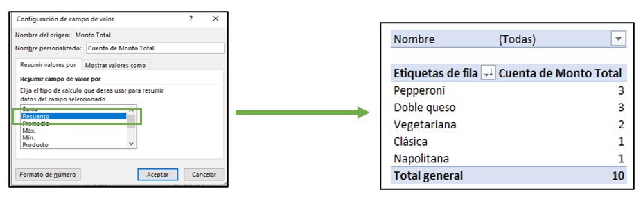
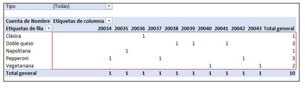
Then a window appears, where it allows us to choose the type of calculation. We select “Count”. In this way, the table is reordered, and we can see, for example, that three of the ten orders that were taken were only for pepperoni pizza.

This video also shows us how to modify our dynamic tables: 

We can also set the number format we need. We go again to “Value field configuration”, but now we go to “Number format”, and we place the “Currency” option, since we are referring to amounts of money in this case.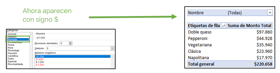

How to filter a pivot table?

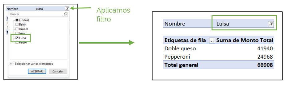
The filter option allows us to select the data that we want to be displayed in our dynamic table, in order to focus our analysis when we have a large amount of data. For example, we want to see only the products that Luisa sold, how do we do it? We go to the “Filter” icon, and select “Luisa”, and we only see the products that Luisa sold!

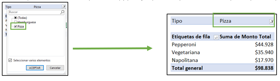
We can also change the type of filter, and for example filter by “Pizzas” in “Type” of product, instead of by “Name”.

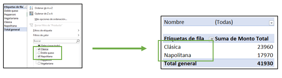
In addition, we can use the same filter as the “Row Labels”, and only select the products with the lowest amount, in this case, “Classic” and “Neapolitan”, looking like this:

What are two-dimensional pivot tables?

We can still get more out of this wonderful tool, we can put much more data in our dynamic tables and enhance their analysis capacity: we can make it two-dimensional, how? We add fields in both rows and columns.

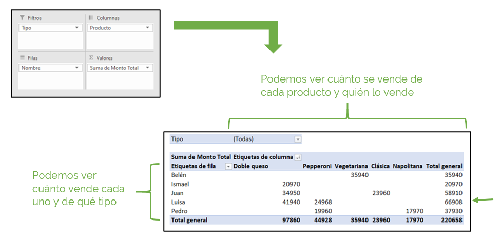
In our example, we take “Type” to “Filter”, “Product” to “Columns”, “Name” to “Rows” and keep “Sum of Total Amount” in “Values”. And now in our dynamic table, we can see that Luisa is the one that sells the most in terms of total amount, and in addition, we can see what products and what amounts she sells!

We can apply all the properties learned from dynamic tables to it in the same way. 

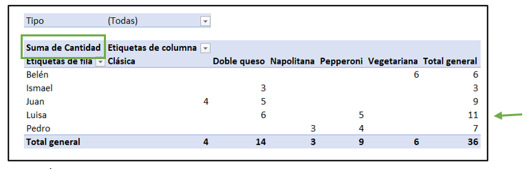
Can drag the fields to make other comparisons. If we now put the “Quantity” in “Sum of Values”, we can see that Luisa is also the one that sells the most in terms of quantity of products! Therefore, we can move the fields, and form different dynamic tables, to perform different types of analysis.

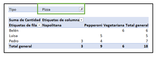
We can also filter, and select to only show the pizzas. And we can see that 18 pizzas were ordered, out of 36 products in total.

What if we want to see all this information together?

That is, we want to see the quantity and total amount of each product, and we also want to see how much each person sold. We take “Type” to “Filter”, “Product” to “Rows”, “Name” to “Columns”, and “Sum of quantity” with “Sum of total amount” to “Values”.

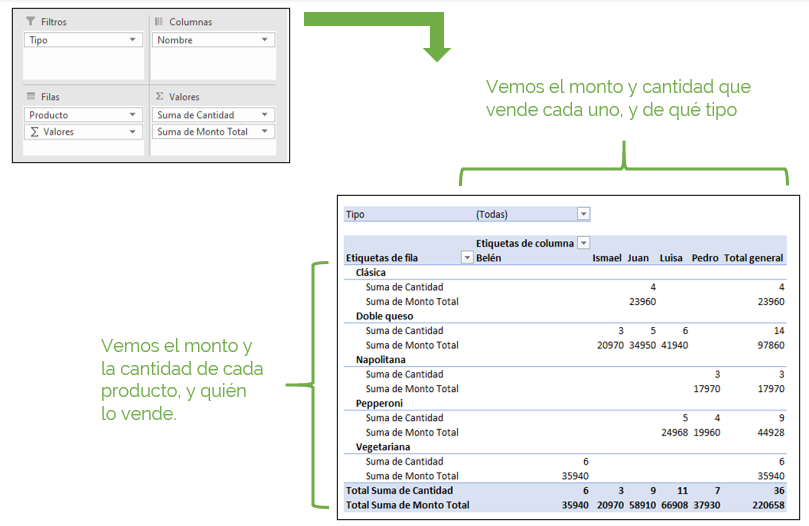
And so we can see all the data we are looking for in a single pivot table, very useful! For example, we can see that Juan sells 9 products, with a total of $58,910, of which 4 are classic burgers, and 5 are Double cheese burgers. On the other hand, we can see that 9 pepperoni pizzas are ordered, with a total of $44,928, of which 5 are sold by Luisa and 4 are sold by Pedro.

Examples of pivot tables

Example 1

Suppose we have a list with all the expenses incurred in three homes in the months of July, August and September. We want to know the total household expenditure each month. 

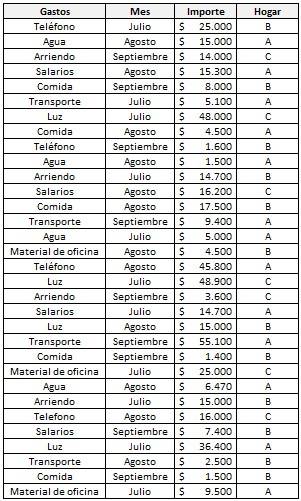
For this, we must make a dynamic table that gives us the sum of all expenses per household in each month.

1. We select the table and in the Insert tab we click on “Dynamic table”.
2. Within the list of fields, we only need the month, the amount and the household, therefore we put the ticket in them. The type of expense incurred does not interest us for what we are looking for, so we should not put a ticket on it.

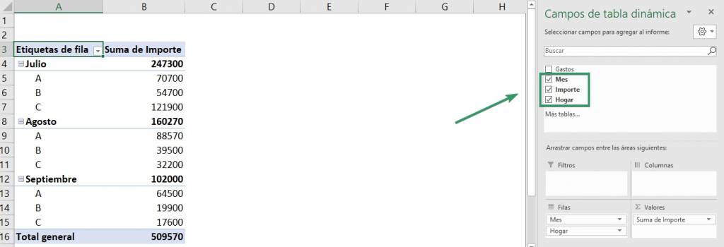
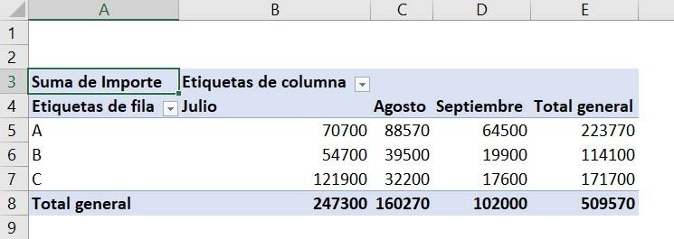
3. We can see that we already have the information we were looking for, but we can arrange our pivot table so that it looks better visually. To do this, we drag the months field into the columns, leaving only the home in the rows. 

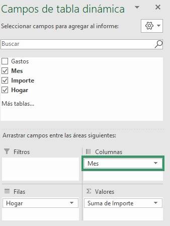
4. Ready! Now we can better see what each household spends per month.

Example 2

We have the following database of a company with the salary of a group of workers and we want to find the salary of a group of workers according to the work area and their age.

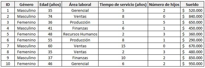
1. We select the table and in the Insert tab we click on “Dynamic table”.
2. Within the list of fields, we only need the salary, age and work area, therefore, we put the ticket in them.

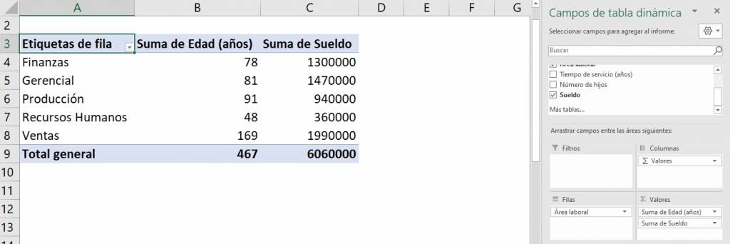
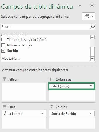
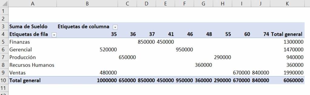
3. We can see that we already have the information we were looking for, but the information is poorly ordered since, for example, the age of the workers was added and we do not want that. To do this, we must drag the “Sum of Age (years)” from the values field to the columns field.

4. Ready! Now we can know the salary of groups of workers according to their age and work area.

Example 3

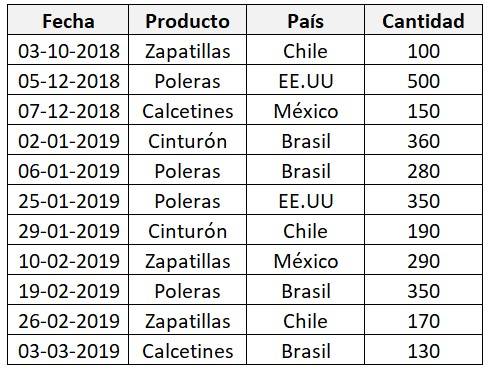
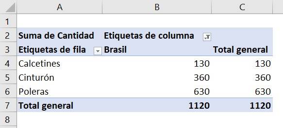
We have data on the export of four products to different countries: Chile, Argentina, USA, Brazil and Mexico. We want to know how many products of each type have been exported to Brazil.

1. We select the table and in the Insert tab we click on “Dynamic table”.
2. Within the list of fields, we only need the country, the product and the exported quantity, therefore, we put the ticket in them.

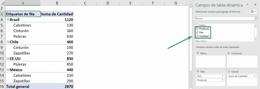
3. We can see that we already have the information we were looking for, but we only need the information for Brazil, so we must drag the Country field to the column field.

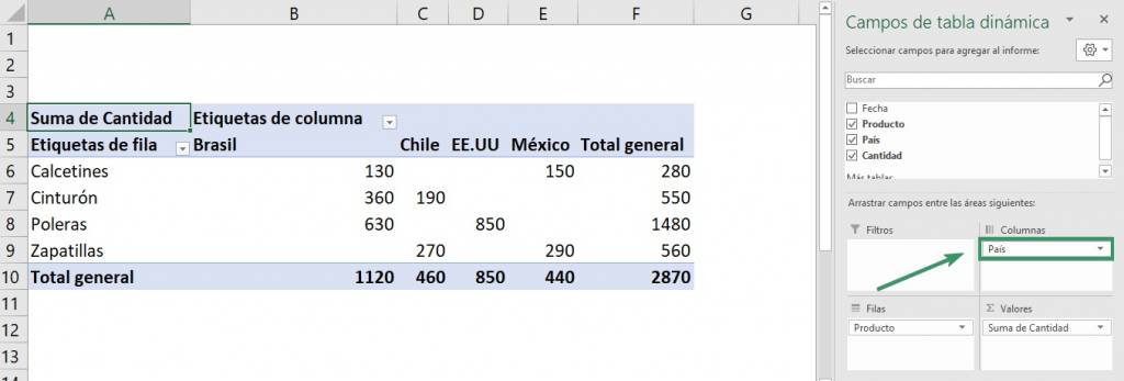
4. Now, we must filter the column and leave only Brazil. For this, we must click on “Column Labels” and obtain the ticket for all countries except Brazil. And select Accept.

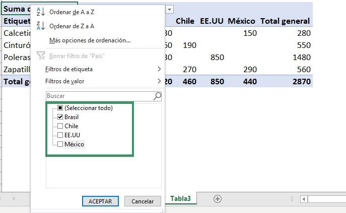
5. Ready! Now we can know the quantity of each product exported to Brazil.

Common errors in pivot tables

Enter all data into pivot tables

A pivot table can include all the fields we want, but it does not mean that we must necessarily include all of them, but rather that we must select only those that are really important for our analysis. Otherwise it is ineffective and useless. 

Not knowing how to return to the “Pivot Table Fields” box

We right click on any cell in the table and then select “Show field list”.

Drag a text field to the values area

In “Values” you can only “Count”, therefore, the dynamic table will give us meaningless information. So, we need to redesign, dragging the text field to the rows or columns area and assign a number field to the “Values” area.

Conclusions

Excel pivot tables are a very useful tool for when we need to group a lot of information from a certain database since it has a great ability to dynamically modify its structure. In addition, it allows you to analyze and compare data in a more complete and easy way.   

Frequent questions

When to use pivot tables in Excel?

When we have a large amount of data and we want to perform a detailed and complete analysis. since dynamic tables allow information to be summarized and ordered, helping to visualize relevant information. 

What are the advantages of using pivot tables?

1. They are easy to use: With just a few clicks you can summarize a large amount of information and display it in different ways.
2. They are dynamic: It is very easy and fast to add and remove fields.
3. You can work in several dimensions: Three dimensions can be used: row, column and filter. 
4. It has multiple views and calculations: It is very easy to change data visualizations.

What steps should I follow to make a dynamic chart?

Ninja Tip: If you want to check or reinforce previous knowledge about graphs in Excel, visit the following post.

Create a pivot chart

1. Select a cell that is within the data table.
2. On the Insert tab, select “Pivot Chart”
3. Select Accept and that's it!

Create a pivot chart from a pivot table

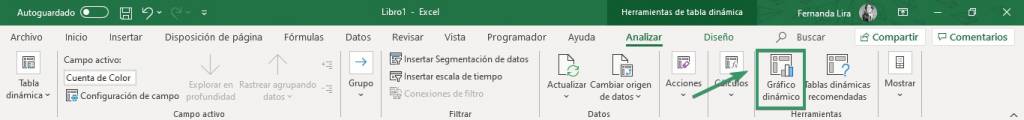
1. Select a cell that is within the pivot table.
2. Under “PivotTable Tools” on the Analyze tab, select “PivotChart”
3. Select the type of graph, click OK and that's it!

Frequent questions