How to make a dropdown list in Excel

Make a dropdown list in Excel is a great way to organize data or arrange items in a cell. Creating drop-down lists in Excel offers several advantages, such as improve efficiency by saving time in data entry and ensure data consistency by limiting input options to a predefined set of values.

Dropdown lists They help organize data in a clear and structured way, and if the data is in a table, the lists They update automatically when items are added or removed. Do you want to learn this and more? Keep reading this Ninja Excel article and discover how to take advantage of drop-down lists in Excel.

What is a dropdown list?

The DROP DOWN LISTS are a feature of data validation in Excel. A dropdown list in a cell is a menu or list which opens and displays the different values to fill the cell. So, when you select an item from the list, The cell is filled automatically.

• Purpose: Automate and facilitate the filling of cells by limiting the options or elements when filling the cell.
• Advantages: Data entry is faster and errors are avoided by restricting the value of a cell to the items in a drop-down list.
• Use: When filling out a cell that has a drop-down list associated with it, you can click on the arrow to the right of the cell to display the list and choose an option or you can type the word yourself. If you choose the second option, it will generally only let you enter the items from the drop-down list.

Items contained in a drop-down list

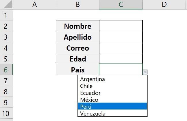
A list contains 4 elements. The following figure shows each of them.

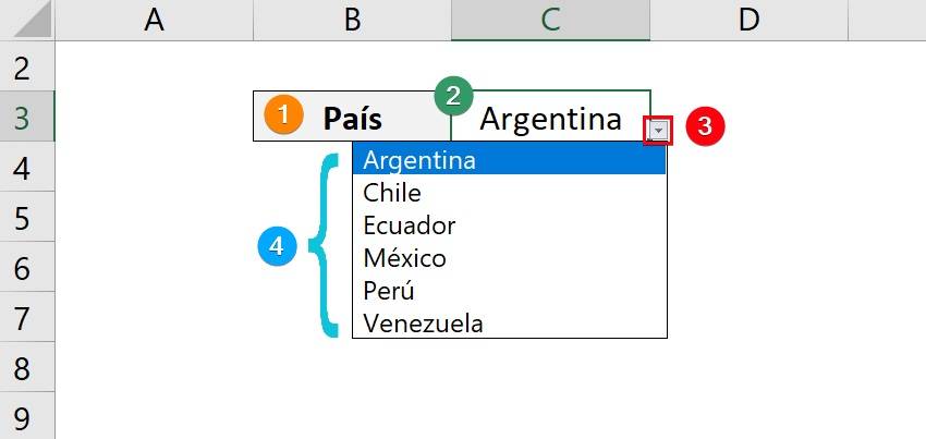
1. Dropdown List Theme

It shows us to which category the elements found within the list belong. In this case, The theme is “Country” Therefore we know that different countries will appear within the list.

2. Cell containing the dropdown list

In this cell is the list, so if we do click in some option, will appear in this cell.

3. List button

It tells us that in the cell there is a drop-down list, if we click on the button aIt will look like a list with all the available options.

4. Options list

It is a window that indicates the different values of the list and of which only one can be chosen.

How to insert them?

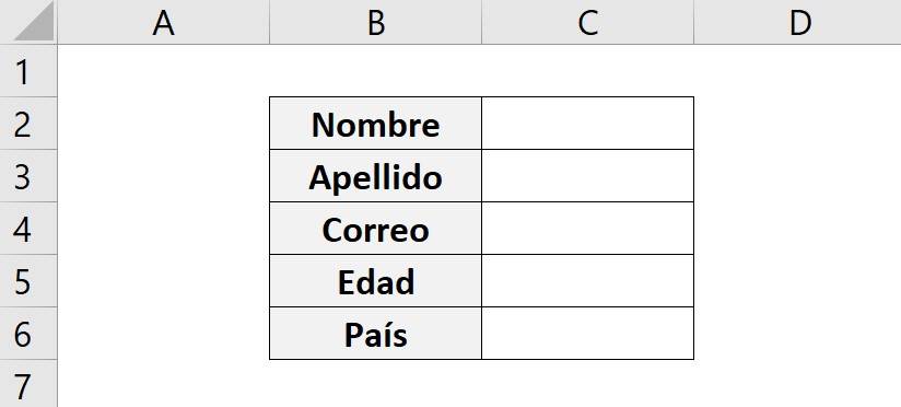
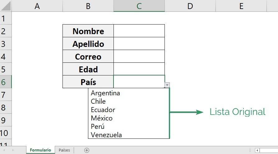
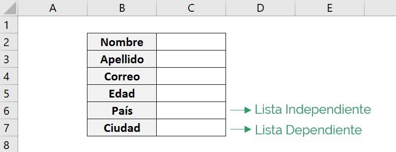
Consider that you have a form in which each person must fill out their information and you want the “Country” section to have only certain options.

1. Open the Excel spreadsheet

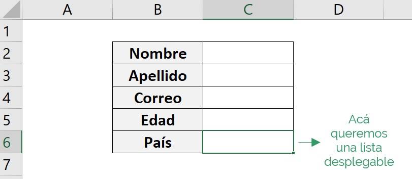
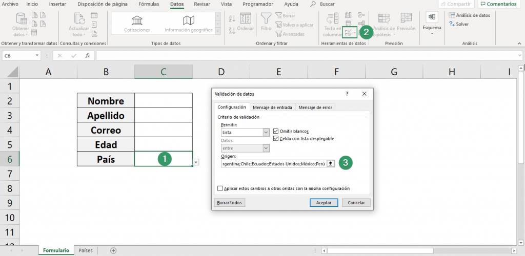
2. Select the cell or cells in which you want to create your list. In this case, we select cell C6 since that is where the country should go.

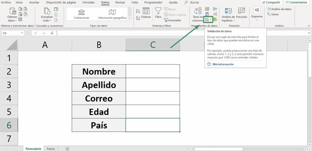
3. Click Data > Data Validation.

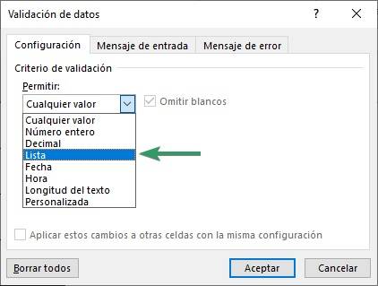
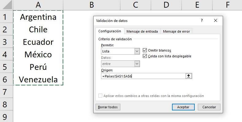
4. In the “Data Validation” dialog box, click on “List”.

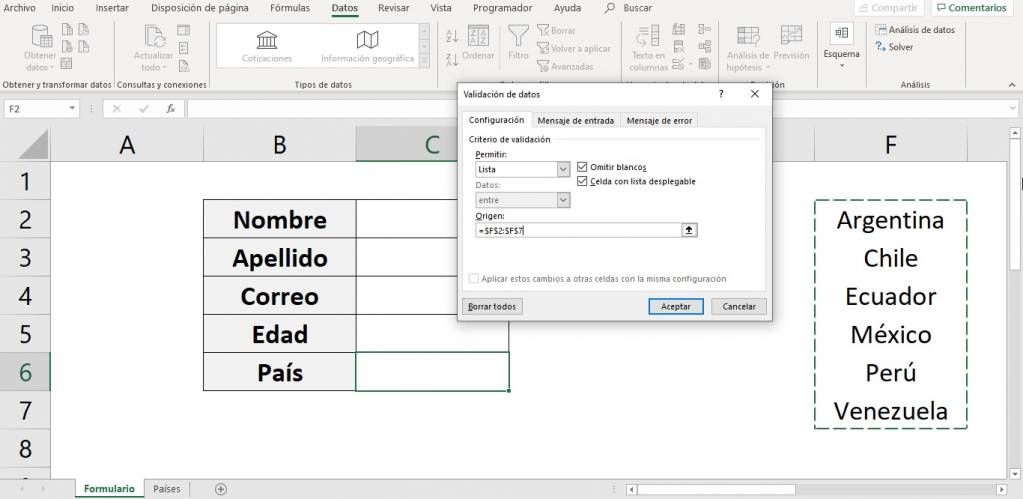
5. Next to “Origin” you must insert the options that will be found in the list, choose an option:

• List from an interval: Choose the cells you want to include in the list.

• Item List: Enter the elements separated by semicolons and without spaces.

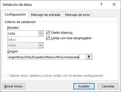
Tip Ninja: Note that when entering the options by writing them manually in “Origin”, the list becomes case sensitive.  So when entering “Argentina” Excel will show us an error saying that what was entered is not in the predefined list. To avoid this, we recommend using the option to add the cells that contain the data.

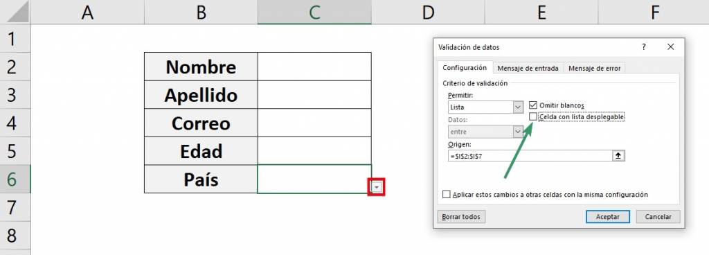
6. The selected cell will have a down arrow. To remove it, uncheck “Cell with drop-down list”.

7. If you enter data in a cell that does not match any item in the list, a notice will appear. If you want users to be able to enter list items, select “Error Message,” then uncheck “Show error message if invalid data is entered.”

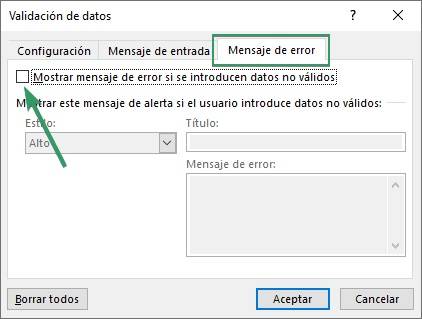
Ninja Tip: In the same “Error Message” tab you can choose the “Style” of the message. If you choose “Warning” or “Information” It lets you enter an item outside the list but with a warning or information window, respectively.

8. Click “Accept”. Ready! To change the color of a cell based on the selected option, use conditional formatting.

Tip Ninja: If you want to learn how to use the conditional format, we recommend you visit this blog.

If you have any questions about how to create a drop-down menu in Excel, we recommend watching the following video.

How to modify a dropdown list?

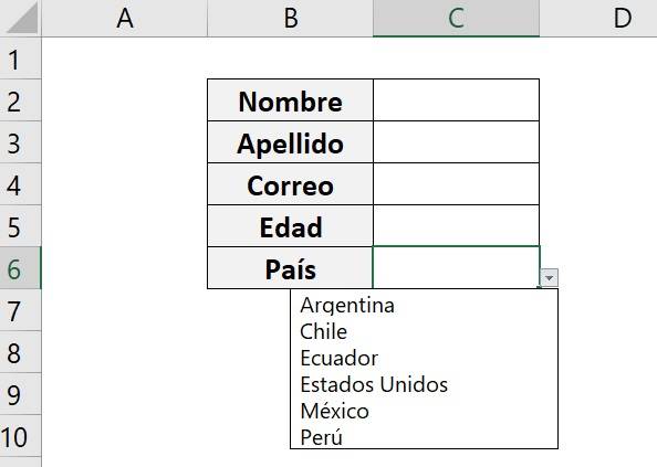
Excel allows you to modify the drop-down lists created. In our list of countries, we want add “United States” and delete “Venezuela”, for this you must follow the following steps:

1. Select the cells you want to change, in this case, the cell that contains our drop-down list.
2. Click Data > Data Validation.
3. To change the options that appear, modify the items next to “Origin.” In this case, we eliminate Venezuela and add the United States.

4. Click on “Accept” That's it, it's already modified!

How to hide source data?

When you create a list from data that is in cells, but you do not want it to be visible, you must follow the following steps.

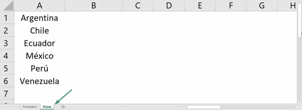
1. The data you will enter in the drop-down list should be in a new tab. In the form, we write the list of countries in the tab called “Countries”.

2. You create the dropdown list using the data from the created tab.

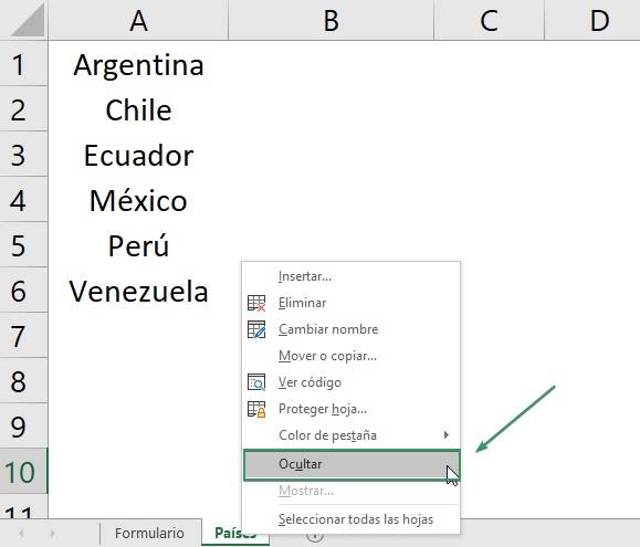
3. Now, we need to hide this new tab. Right click on the tab name and click “Hide”.

4. Ready, you now have your form with the list of data hidden!

Delete a dropdown list

To delete a drop-down list from Excel you must follow the following steps:

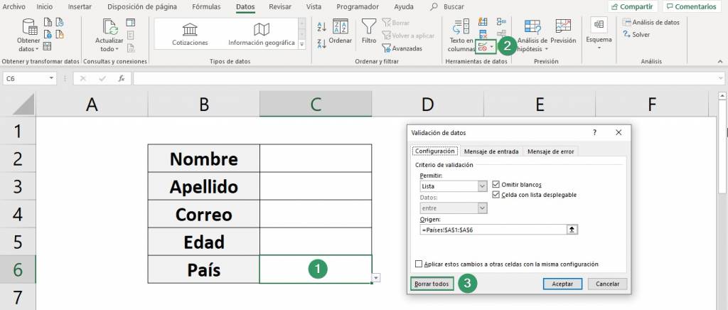
1. Select the cell where you have the dropdown list. In our example, cell C6.
2. Go to the “Data” tab and click on “Data Validation”.
3. Select “Delete all” and click “OK”.

Tip Ninja: If you want to delete all cells with drop-down lists you can click on “Apply these changes to other cells with the same configuration” in the same data validation window.

Dynamic dropdown list

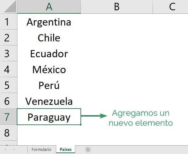
There is a formula you can use to have the drop-down list expand automatically when you add an item to the end of the data list.

1. Go to the sheet where you have the form and click on the cell where we want to create the drop-down list. In this case it is C6.
2. In the “Origin” section write: =OFFSET('Countries'!$A$1;0;0;COUNTA('Countries!$A:$A);1)

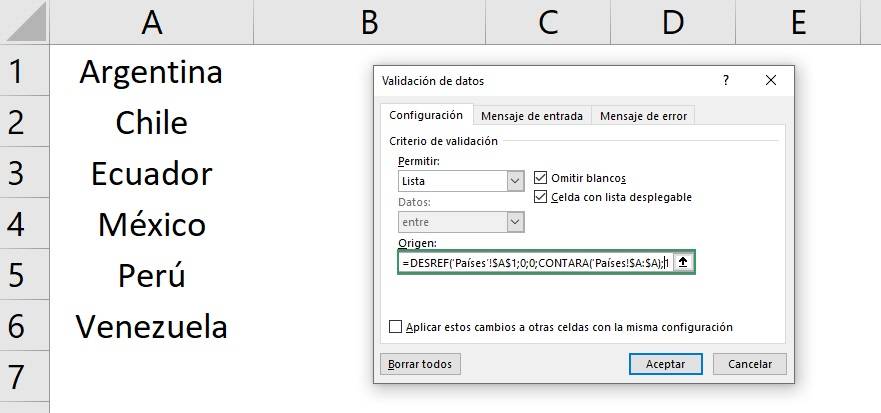
3. Click “Accept”.

What does the OFFSET function do?

The RESREF function (OFFSET in English) in Excel returns a cell or set of cells for a defined number of rows and columns.

Syntax: RESREF(reference; rows; columns; [height]; [width])

• reference: cell from which to select
• rows: is the number of rows, up or down, that you want the cell to reference.
• columns: is the number of columns, to the right or left, that you want the cell to reference.
• [height]: is the height, in number of rows, that you want the reference to have. It's optional.
• [broad]: is the width, in number of columns, that you want the reference to have. It's optional.

What does the COUNTA function do?

The COUNTA function (COUNTA in English) Counts the number of non-empty cells in an interval.

Syntax: COUNT (value1;[value2];…)

• value1: cell from which to count
• value2,…: other values that you want to count. It's optional.

In this way, when writing OFFSET('Countries!$A$1,0,0,COUNTA('Countries!$A:$A),1), we mean:

• reference = 'Countries!$A$1: Select A1 from the countries option sheet (reference)
• rows = 0: Do not move up or down
• columns = 0: Do not move sideways
• height = “COUNTA('Countries!$A:$A)”): the length of the column must be the number of non-empty cells in column A.
• width = 1: Only one column.

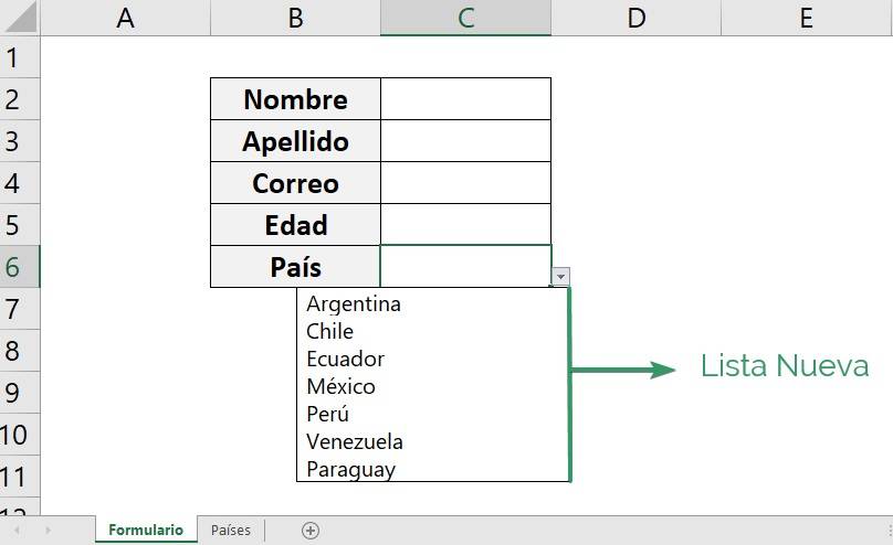
6. So, when you add elements below the original, they will automatically be added to the drop-down list

Dependent dropdown lists

An advanced and very useful practice is to make dependent dropdown lists. This is a dropdown list that depends on the option chosen from another previous dropdown list.

For example, in the same form as in the previous exercises, now you want to add the item “City”, but you want a different list to open if Chile is chosen or Mexico is chosen.

To create a dependent dropdown list follow these steps:

1. In a separate table or a different sheet than the form, you must fill in the options for both country and city.
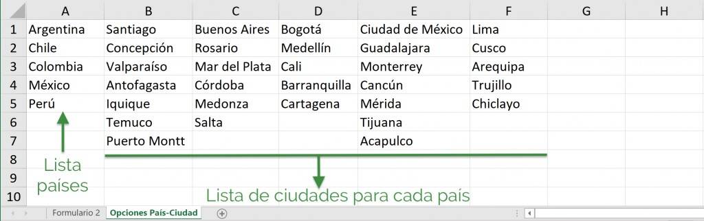
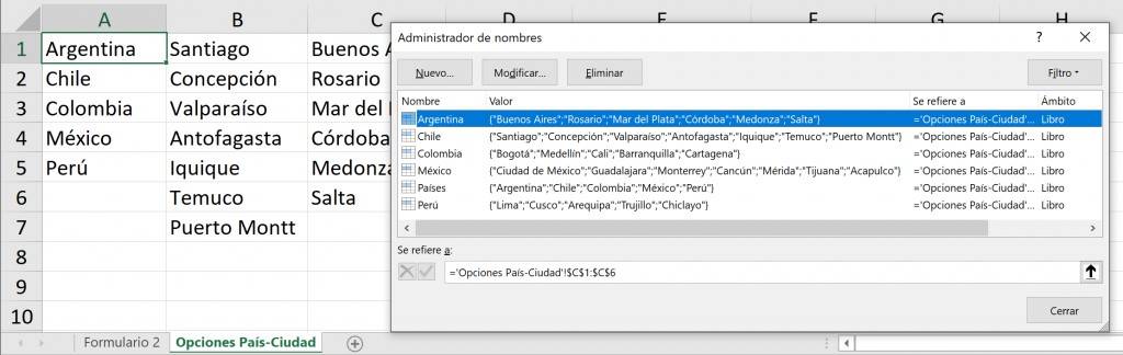
2. Assign a name to each range (set) of cells:
   1. To do this, select one of the lists. For example, select all countries.
   2. Go to the “Formulas” tab and do click in “Assign name”.

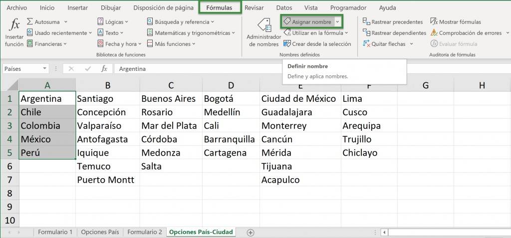
3. Give it the name of the list. In this case it would be “Countries”. Click on "Accept".

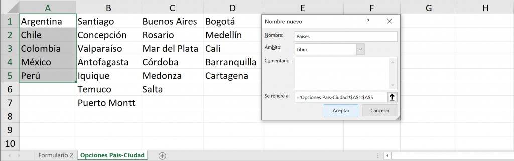
4. Do the same for all lists. If you click on “Name Manager” you can see all the ranges of cells that you assigned names to.

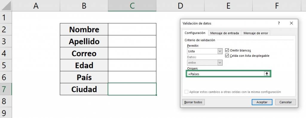
3. Now, select the cell from the dropdown list "mother" (on which your answer depends the other list). In this case it is C6, which is for filling in countries.
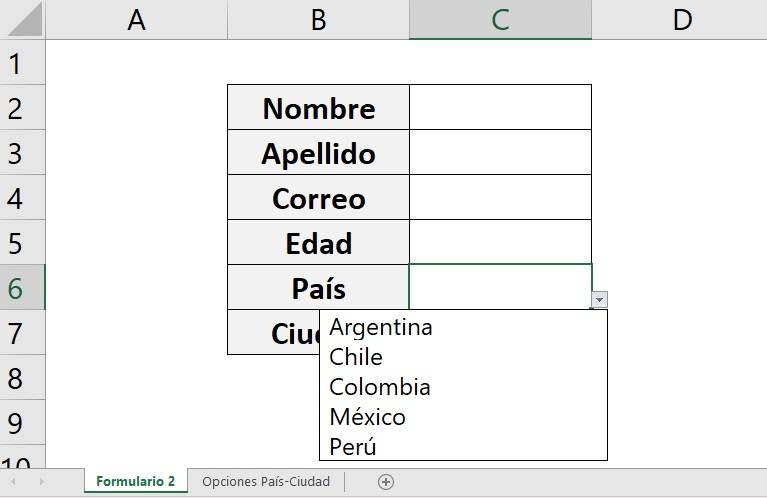
4. Create the dropdown list and in the section “Origin” writes “=Countries” and click “Accept”.

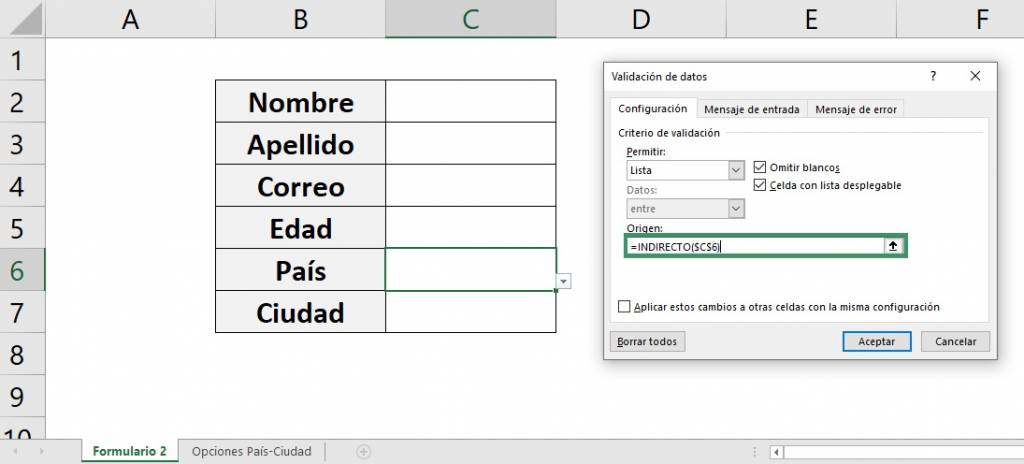
5. Now, create the drop-down list that we want to depend on the response of the previous drop-down list. In this case it is C7, which is for filling cities.
6. Go to the tab “Data” and click on “Data validation” and choose “List” in the “Allow” section.
7. In the “Origin” section write “=INDIRECT($C$6)” and click “OK”.

What does the INDIRECT function do?

The INDIRECT function converts text to a valid cell reference. Thus, it obtains the value of the Countries cell, such as “Chile” and makes Excel read it as the range called Chile, thus displaying the same list.

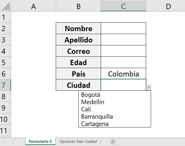
In this way, if we choose Colombia as the country, then the following list is displayed:

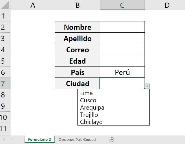
If we choose Peru, then this list is displayed:

Frequent questions

How to copy and paste a dropdown list in Excel?

If you want to apply the drop-down list to multiple cells, you just have to select the cell that contains the list and drag from the lower right corner to the rest of the cells. This way it will be applied to all cells.

How to list a list in Excel?

To list them, we must type all the options from the drop-down list in a new Excel tab and then, when creating the drop-down list, select it.

This list of data can be sorted alphabetically, numbered with ascending numbers, in order, and many more options.

In the following video you will see how to copy a drop-down list, as well as see how to make a drop-down list from a list of data.

Frequent questions