How to make an amortization table in Excel?

Amortization refers to the process in which we begin to pay off the debt of a loan until it is completely paid off. In that sense, an amortization table in Excel will allow us to know how the payments we make are distributed or how many installments remain.

What is an amortization table?

An amortization table is a table that shows a history where we can see in detail the payments made, the missing payments and how they are distributed to settle a loan.

What are amortization tables for?

The use of an amortization table will allow us to have a complete view of any credit. Thus, with the information it provides we can be prepared to face the costs of applying for a loan and maintain adequate control of the entire process.

What elements should an amortization table contain?

When calculating an amortization table in Excel we must consider the following concepts:

• Period: times in which installment payments must be made.
• Interest: consideration that the lender receives in each installment. 
• Amortization or payment of capital: it is the net amount that is aimed at reducing the capital of the debt in each installment. It does not consider interests.
• Fee to pay: it is the total amount that must be paid in each period. 
• Balance: This is the amount that remains to be paid and is reduced after each installment, until the loan is paid off.

How to create an amortization table in Excel?

Creating an amortization table involves knowing some variables to calculate the payment through 3 Excel functions.

Variables to calculate payment

There are 3 variables whose values we need to manage for the correct calculation of the payments we will make. We detail them below.

Credit value

It refers to the net amount of credit that we receive from the financial institution or lender.

Interest rate

The interest rate represents the profit that the financial institution obtains after granting the loan. When we pay, we cover the amount we receive and also an additional amount for the services provided by the institution. 

Payment amount 

This variable refers to the number of installments that we will pay to cover the interest and principal in order to pay off the loan.

Functions in Excel to calculate payment

The variables that we mentioned before are necessary to carry out the calculations with the functions: PAGO, PAGOINT and PAGOPRIN. Each Excel formula for the amortization table will return an amount related to interest, principal payment, and monthly payments.

PAYMENT Function

Through the PAYMENT function we will obtain the amount that we must pay monthly to cover our loan. Its syntax is:

=PAYMENT(monthly interest rate, number of payments, credit value)

=PAYMENT(1%,12,100000)

PAGOINT function

With the use of the PAGOINT function we can know the amount corresponding to the monthly interest of each installment we pay. Its syntax is:

=PAGOINT(interest rate, period number, number of payments, credit value)

=INTPAYMENT(1%,2,12,100000)

PAGOPRIN function

The PAGOPRIN function allows us to determine the amount corresponding to the capital payment in each of the installments we pay. Although it uses the same variables as the PAGOINT function, the operation returns the amount that is added to the capital. Its syntax is the following:

=PAGOPRIN((interest rate, period number, number of payments, credit value)

=INTPAYMENT(1%,2,12,100000)

Examples of amortization table in Excel

Loan modalities may vary according to the way in which payments are made or whether the interest is fixed or variable. In that sense, we are going to present some examples of amortization tables for different cases.

Amortization table in Excel for a bank loan

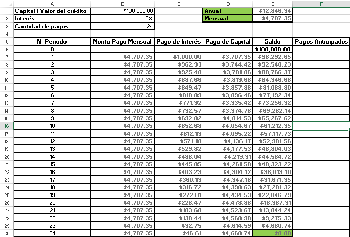
For this example of a bank credit amortization table, we request a loan of $100,000.00 at an annual interest rate of 12%, to be paid in 24 installments. 

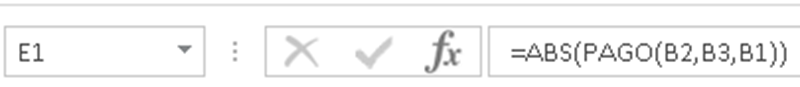
We will use the PAYMENT function to calculate the annual and monthly payment amounts.

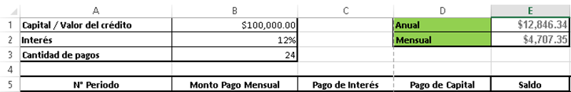
The annual payment is calculated by selecting the variables Interest, number of payments and value of the credit. For its part, the monthly amount is obtained with the same function, but dividing the interest by 12. It would look like this:

Annual payment:

Monthly payment:

Using the ABS function allows you to obtain the result in positive numbers.

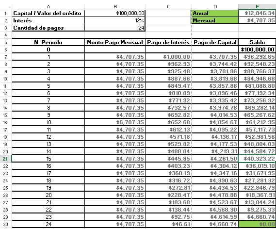
Now we move on to creating the table for the breakdown of payments. To do this, we generate 4 new rows and enable as many columns as payments must be made, in this case 24. The new rows will be: 

• Period number: month number corresponding to a quota.
• Monthly payment: amount obtained through the PAYMENT function.
• Interest payment: amount obtained with the PAGOINT function.
• Capital Payment: amount obtained with the PAGOPRIN function.
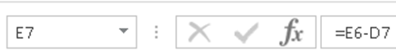
• Balance: progress of credit payment obtained by subtracting the balance of the previous period and the current capital payment.

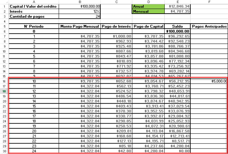
Amortization table in Excel with advance payments

When we receive a loan, the situation may arise where we want to anticipate the payment of a certain period. 

Continuing with the previous example, we can adapt our bank credit amortization table so that it supports the calculation with advance payments. To do this we must make a series of changes:

• Add a new row before period one, to create period zero.
• Insert the amount from the credit value cell in the first cell corresponding to Balance.
• Create a new column identified as advance payments.

We will apply the penultimate change by editing the monthly payment formula and it would look like this

.

In the second block of the formula we are subtracting the period number from the number of payments and in the third, we point to the balance of period zero. At the end, we add the advance payments cell. 

Finally we have to replace the interest payment and principal payment formulas with their conceptual calculations. It would be like this:

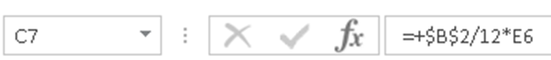
Interest payment: monthly interest rate multiplied by the balance of the previous period.

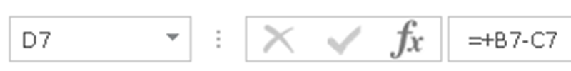
Principal Payment: Interest payments are subtracted from the monthly payment amount.

Drag the formulas down to fill in the rest of the cells and then you can enter your advance payments.

Amortization table in Excel with fixed fee

The first case that we propose is also an example of an amortization table in Excel with a fixed fee. This is because the monthly payment represents an invariable amount, so the PAYMENT, PAGOINT, and PAGOPRIN functions work very well for these calculations.

Related questions