Correlation coefficient in Excel: How to calculate it

Key information

The correlation coefficient - also known as “Pearson's correlation coefficient” - is a measure of the relationship that exists between two variables, that is, how one moves due to movements in the other. In Excel it can be calculated mainly in two ways, depending on whether we want to obtain the correlation between only two variables or if we want to obtain the correlation matrix between several pairs of them.

What is correlation?

The correlation between two variables is the proportional relationship that exists between them, that is, how one changes due to changes in the other. For example, we might expect there to be some relationship between a company's revenues and costs. Most likely, in this case we have a positive correlation, since the higher the income, the higher the costs as well.

To measure the correlation we work with the correlation coefficient, which can take a value between -1 and 1 depending on the different relationships that exist between two variables.

If the variables have a correlation coefficient of 1, it means that they have a perfect positive correlation. When one variable increases, the other also increases. When one variable decreases, the other does too. To understand what we mean, let's look at the following example in which we have the income and costs of a company:

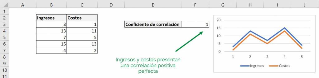
We can see in the example that as revenue increases, costs also increase, which is clearly reflected in the line graph.

Ninja Tip: The correlation coefficient is widely used to see the correlation of two variables over time, so it is very common for it to be accompanied by a line graph to make it easier to illustrate the relationship. If you want to learn how to make a line chart in Excel easily you can go to the following article. If you want to learn how to make other types of graphics, click here.

On the other hand, if the variables have a correlation coefficient of -1, it means that they have a perfect negative correlation (also known as an inverse relationship). In this case, as one of the variables increases, the other decreases:

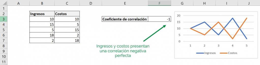
Now in the example the opposite case occurs than in the last case, as income increases, costs fall in a similar proportion.

If the correlation coefficient between the variables is very close to 0, it means that there is no type of relationship between them and that movements in one variable are not accompanied by changes in the other. In this way, as we approach 0 the relationship between the variables is smaller and is not a constant proportional relationship. Generally correlation coefficients greater than 0.5 or less than -0.5 describe relatively important relationships.

It must be taken into account that the correlation coefficient describes a relationship, not that one variable is having a direct effect on the other. To understand more about this difference click here.

Way 1: Using the CORREL COEF function

The first way to obtain the correlation between 2 variables is to use the function CORREL COEF. This way is the simplest and fastest, but it only allows you to obtain the correlation between a pair of variables at a time:

Syntax:

=CORRELCOEF(matrix1; matrix2)

Arguments:

array1 = Mandatory. First range of cells on which we want to calculate the correlation coefficient. Contains the information of the first of the variables to use.

matrix2 = Mandatory. Second range of cells over which we want to calculate the correlation coefficient. Contains the information of the second of the variables to use.

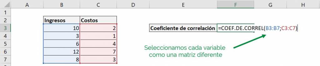
Going back to the example of our company's revenues and costs, all we have to do is select our first variable, in this case “Revenue”, as our array1 and our second variable, the “Costs”, as the matrix2:

With which we obtain the following result:

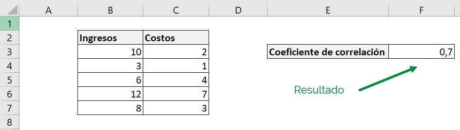
As we can see we have a correlation coefficient of 0.7, which means that income and costs have a positive correlation.

Way 2: Obtaining several correlation coefficients at once

The second way to obtain the correlation coefficient is a little more complex, but it allows us to obtain in the same calculation the different correlation coefficients between more than one pair of variables.

Activating the tools to calculate the correlation coefficient in Excel

The first step when trying to calculate correlation in Excel with this method is to make sure we have the tool called “Data Analysis” activated. For this we do the following:

Step 1: We click on the “File” option in the main Excel bar:

Step 2: In the left sidebar we click on “Options”.

Step 3: A new window will open, in which we click on “Add-ons”:

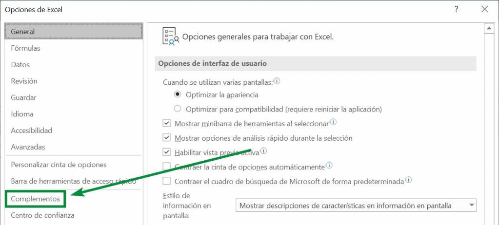
Step 4: In the add-ons window we click on the “Go” box:

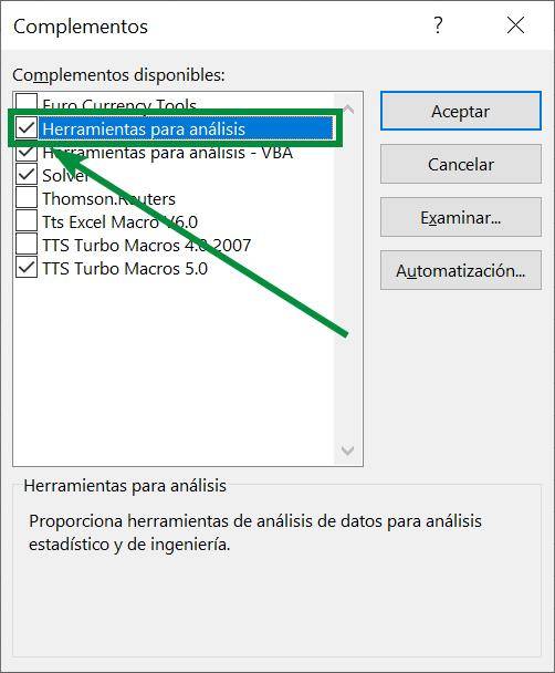
Step 5: A new window will open, in which we must make sure that the “Analysis Tools” option has a ticket in the box to its left. After this we click on “Accept”:

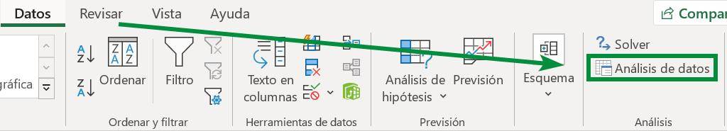
Step 6: If we carry out all these steps correctly, the “Data Analysis” tool should be in the “Data” tab of the main Excel bar, in the “Analysis” section:

Using “Data Analysis” to calculate correlation coefficients

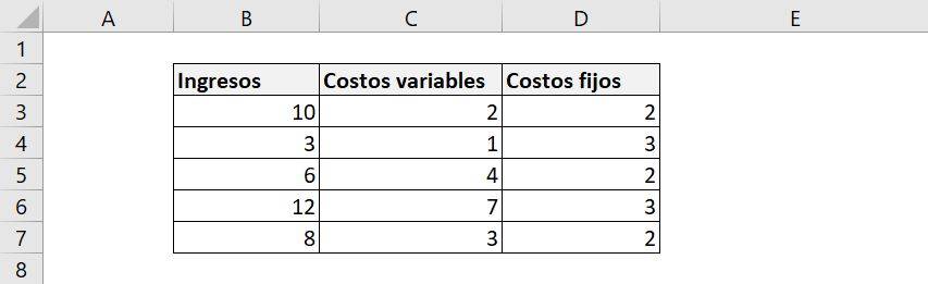
Now to calculate the correlation coefficient in Excel using the “Data Analysis” tool, let's look at an example similar to form 1, but now including that we have both variable costs and fixed costs:

Step 1: We click on the “Data Analysis” tool, which will open the following window:

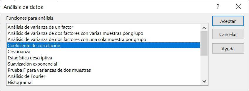
Step 2: We select the “Correlation coefficient” option and click on “OK” (we can also double click), which will open the following window:

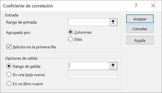
Step 3: In the “Input Range” section we indicate where our data is located, making sure to include the variable names in the cell selection. To make this process easier we can click on the black arrow on the right and select the cells manually:

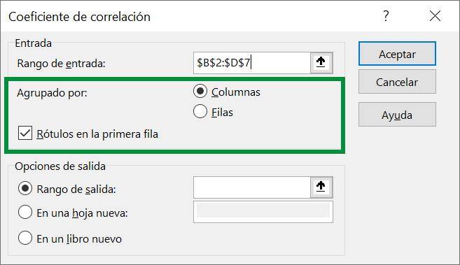
Step 4: Now we indicate in “Group by” that our variables are in different columns, selecting the “Columns” option. Additionally, we indicate that the variable names are in the first row, with the “Labels in the first row” option:

Step 5: The last thing left to do is indicate where we want Excel to give us the table with the different correlation coefficients. In this case we want it to appear in cell F2, so we select that cell:

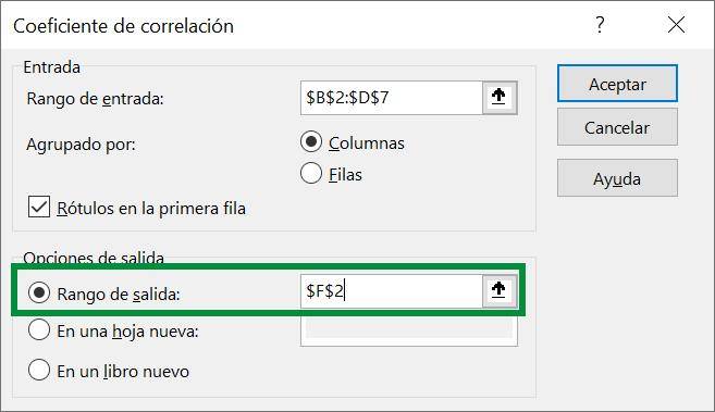
Tip Ninja: Let's keep in mind that the table that Excel gives us occupies more than one cell, even if we indicate only one cell, so we must make sure that we have enough space so that the output table does not overwrite information that we have.

Ready! By clicking on “Accept” the information we are looking for will appear, in what is known as “Correlation Matrix”:

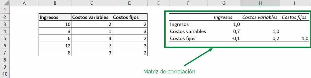
To see the correlation coefficient between two variables, you only need to go to the table and see where the row of one intersects with the column of the other. For example, if we want to see the intersection between “Revenue” and “Fixed costs”:

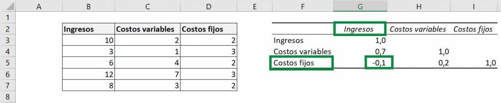
We can see then that the correlation coefficient between these two variables is -0.1.

Ninja Tip: The “Data Analysis” tool allows you to access other very useful statistical functions in Excel. One of the most important is regressions. If you want to learn how to do regressions in Excel you can go to the following article.