How to compare two columns in Excel

Key information
COMPARE TWO COLUMNS In Excel it is simply finding what things are in common, and what things are not, between one column and another. It is very useful when you have information that comes from different sources and you need to verify if they have elements that are the same or if they are different. For example, let's say you have data for countries with their capitals, and you have other data with countries and their continent. You would like to put everything together in a single spreadsheet to have continent, country and capital. The problem is that you suspect that one base has more countries than another and also that there are some that are written differently. One way to match the information is by comparing the columns and seeing which elements are different, in order to consolidate all the information in a single table. We will see it below in more detail.
The basics
There is no single way to compare columns in Excel. To make sure you find the answer to what you need, you should ask yourself the following questions.
Do I need to compare within the same row of columns?
If the answer to this question is yes, then you should go to the first section of this post: Compare two columns with exact row matching. This way, you will be sure to find the same and different elements of cells that are next to each other.
If the answer is no, then go to the next question.
Do I care about the position of the data in the columns I'm comparing?
If you got this question, it's because the answer is no. In this case, you probably want to compare the elements in one column with the elements in the other in general terms, regardless of whether or not they match in terms of adjacent cells. To do this, go to the Compare two columns to identify duplicates or Compare two columns to identify differences section, depending on what you want to identify.

Compare two columns with exact row match
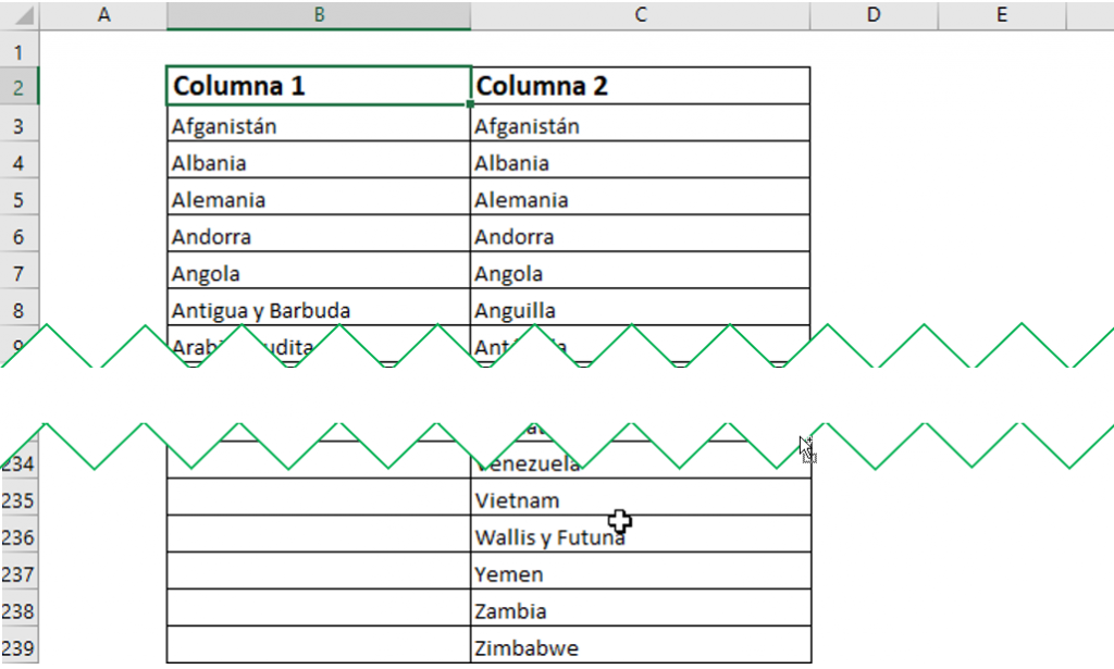
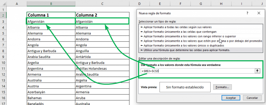
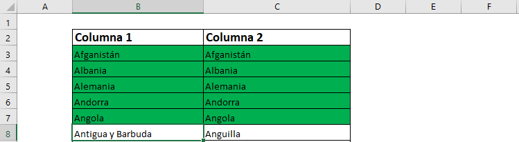
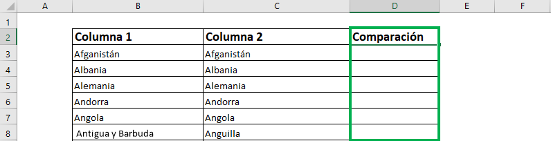
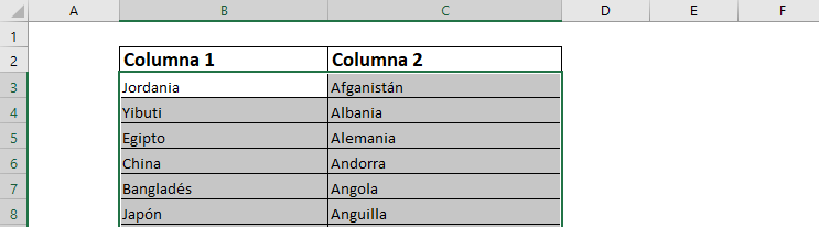
Let us assume the following list of countries arranged alphabetically. Each column comes from different sources and therefore we seek to see which countries are found in both sources and which countries only in one. As seen in the image, the second column is longer and therefore contains more countries, making a comparison crucial to understand the differences.
Highlighting matches with conditional formatting
Let's say we want to highlight those rows that contain exactly the same information in each of their columns.
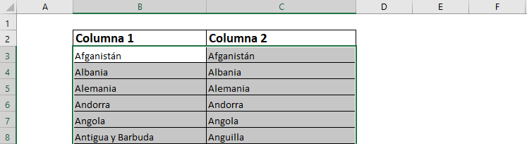
Step 1: Select all the cells where you want to find the matches and differences. Include titles only if you want to find matches there as well.
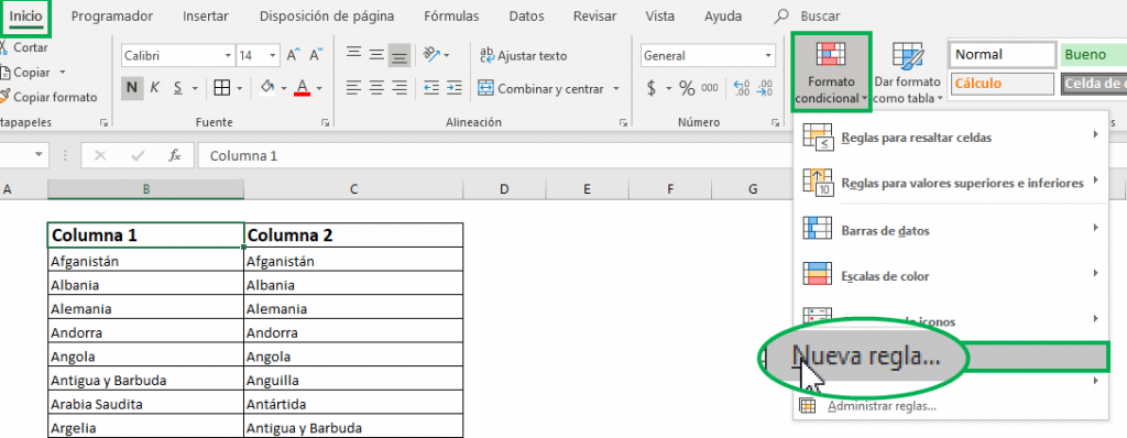
Step 2: On the “Home” tab, in the “Styles” section, click “Conditional formatting” and then “New rule.”
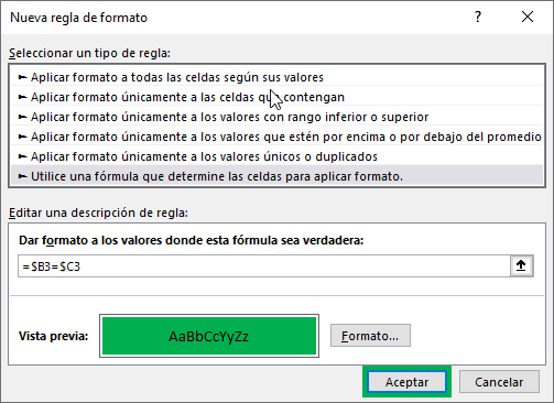
Step 3: A new window will appear. In the “Select rule type” box, click on the last option that says “Use a formula that determines the cells to apply formatting.
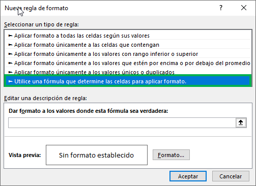
Step 4: In the same window, you must indicate which cells you want to format. Click the box under “Format values where this formula is true.” Since we want matches, we need the first cell in the first column to be equal to the first cell in the second column, that is:
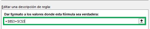
To achieve this, you can write it or click on the cells to have them written automatically. Remember to write the “=” symbol between each expression to indicate that you want those cells to be equal.
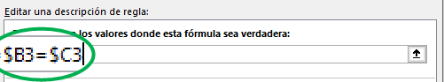
Step 5: Leave only a “$” symbol located at the beginning of the cell name to set the column. This way, the formatting will extend to the rest of the cells in the column.
Step 6: Click the “Format” button to indicate how you want the matches to look.
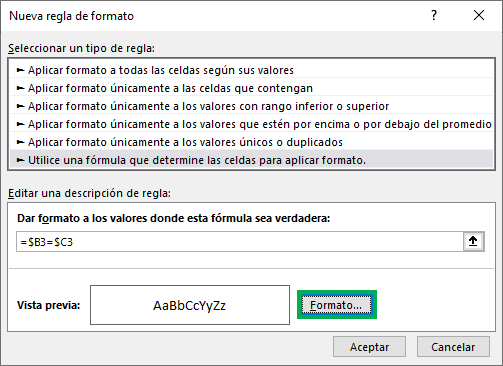
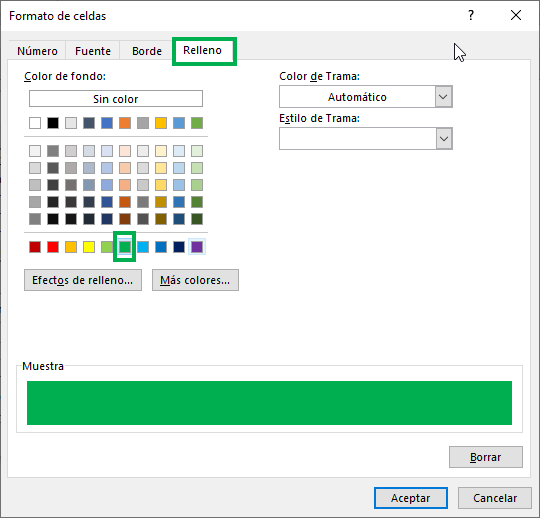
Step 7: Define the format. In this case, we will simply leave a green background by selecting the “Fill” tab and selecting that color. You can also define a font color and a font style. Click “Accept” when finished.
Step 8: Click “OK” again to complete the step of defining the new rule to compare columns.
We see that only the beginning of the table acquired the color, since there is only a match in the first five rows.
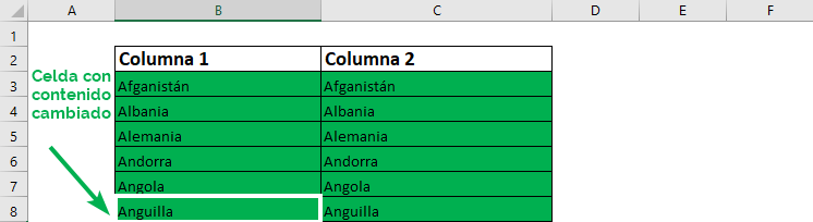
If we change the content of any cell to match its adjacent one, then it automatically takes on the set format.
This is a graphical way of comparing columns since it is observed through colors. Read on to see how to indicate differences and similarities with a column that returns an indicator of the comparison result.
Ninja Tip: If you want to know a little more about how conditional formatting works, you can check out this post.
Pointing out matches with a word
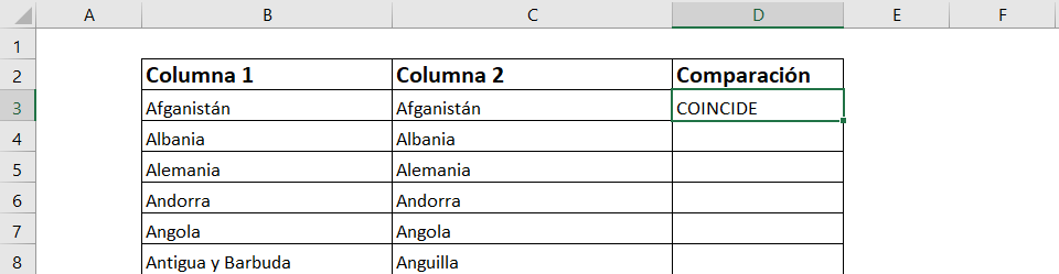
Let's assume the same base as before, but now to compare two columns we will add a new one with the result.
Step 1: Add a new column to the table so that it contains the result of the comparison between columns.
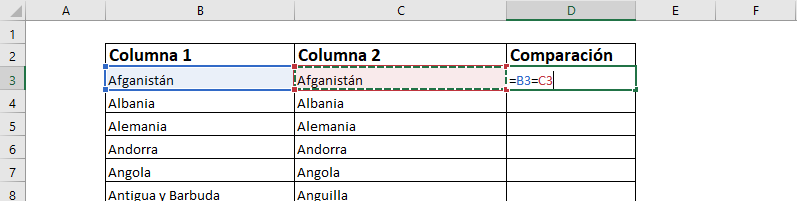
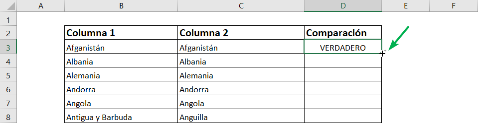
Step 3 (alternative 1): In the first cell of the “Comparison” column, indicate that you want the first cell in “Column 1” to be equal to the first cell in “Column 2,” and then press the Enter key

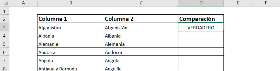
Since the content of the indicated cells does indeed match, the result is the following:
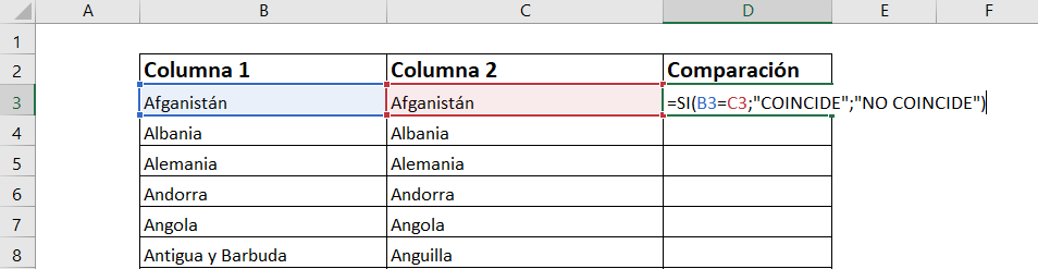
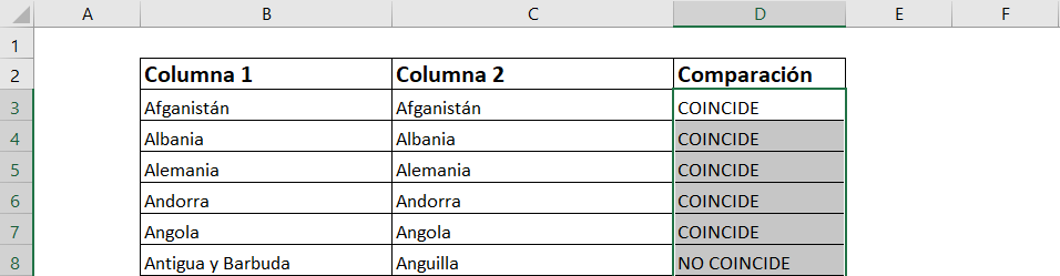
Step 3 (alternative 2): If you would like to specify the text to be displayed when doing the comparison, then you can use the IF function. Indicate that you want the first cell in “Column 1” to be equal to the first cell in “Column 2”, then indicate what you want it to say if the condition is met (“MATCH”), and what if not (“DOES NOT MATCH”). "). Press the Enter key.

The result is as follows:
Step 4: Position yourself in the lower right corner of the cell with the formula until the mouse cursor turns into a black cross.
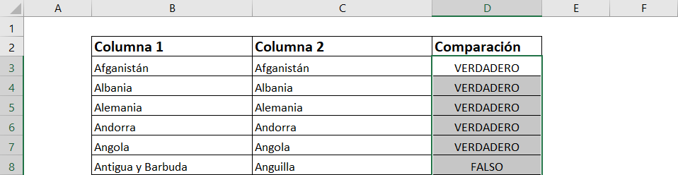
Step 5: Double click so that the formula drags down. The result for each of the cases is the following:
Alternative 1
Alternative 2
Compare two columns to identify duplicates
In case when comparing columns you do not care about the position of the components of each of the columns, but only the content, you can use Excel's conditional formatting to identify duplicates of a base. Notice that now the countries in the first column are out of order, therefore, it is most likely that the contents of adjacent cells do not match, which is not relevant in this case.
Step 1: Select all the cells where you want to find the matches and differences. Include the titles only if you also want to compare the content there.
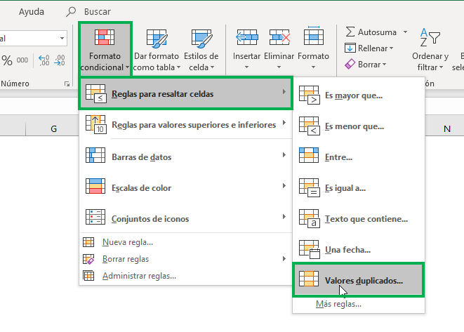
Step 2: In the “Home” tab, in the “Styles” section, click on “Conditional formatting”, then on “Rules for highlighting cells” and finally on “Duplicate values”.
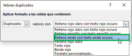
Step 3: In the new window, select the format you want to give to the duplicate cells. In this case, “Green fill with dark green text.” Then select “Accept”.
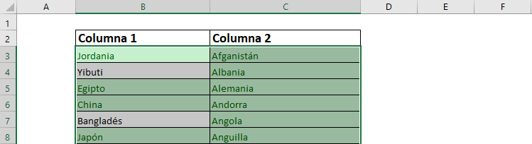
As you can see, the duplicate cells remained in the format established in the previous step. Regardless of the position, the cell is dyed green if in any Elsewhere in the table there is a cell with the same content.
If you want to sort by color, go to Step 4 in the next section to see how to do it.
Compare two columns to identify differences
Now we take the same case as the previous one, but instead of identifying duplicates in the comparison, we identify those elements that are not shared between both columns.
Repeat Step 1 and 2 from the previous section.
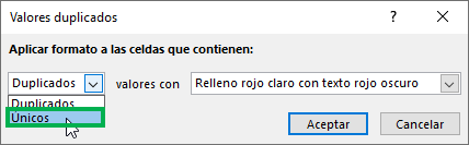
Step 3: In the new window, select “Unique” and then the format you want to give it. In this case, we will leave “Light red fill with dark red text”. Then select “OK”.
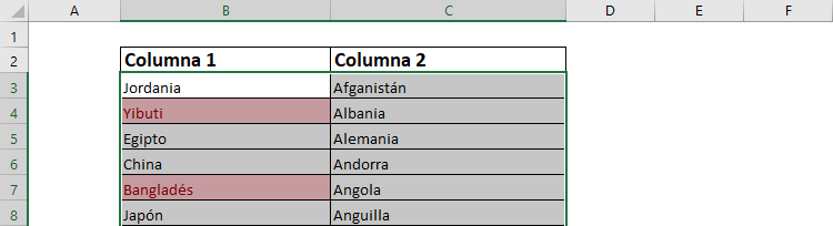
The result is exactly the opposite of the previous case, that is, only those cells are highlighted whose content cannot be found more than once in the selected data.
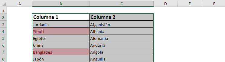
Step 4 (Optional): If you want to see all the different elements together at the beginning of the table, you can ask Excel to sort them according to this criterion.
- Selecciona la columna que quieres ordenar. Puedes querer ordenar ambas columnas, pero deberás escoger solamente una para establecer el criterio de orden. En este caso seleccionaremos ambas columnas con los títulos.
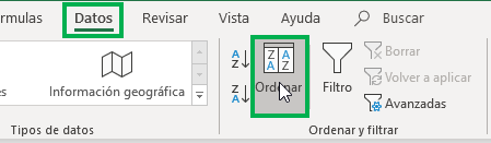
- In the “Data” tab, in the “Sort and Filter” section, click “Sort”.
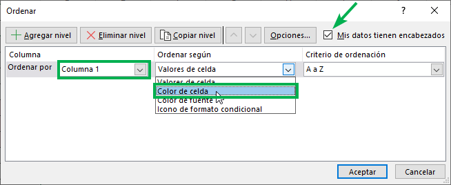
- En la nueva ventana que aparece, selecciona los criterios para ordenar. En este caso, dejaremos que se ordene por “Columna 1”, pero cambiaremos “Ordenar según” a “Color de celda”. Asegúrate que esté chequeada la casilla “Mis datos tienen encabezados” en la esquina superior derecha de la ventana.
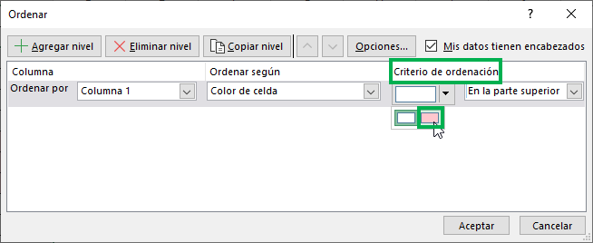
- In “Sort Criteria”, select the color you want to sort (that light red), and then define whether you want it to be at the top or bottom of the table. In this case, we will leave it at the top.
- Finally, click “Accept”. The result is as follows:
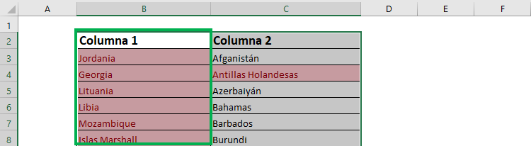
- We see that all the elements with color from “Column 1” were at the top. The same did not happen with “Column 2” since the original rows were maintained, but not their order.
Compare two columns and extract matches
It is also possible to create a new table with the elements that match between the two columns you are comparing. For this you can use the function VLOOKUP or its improved version, the set of functions INDEX-MATCH.
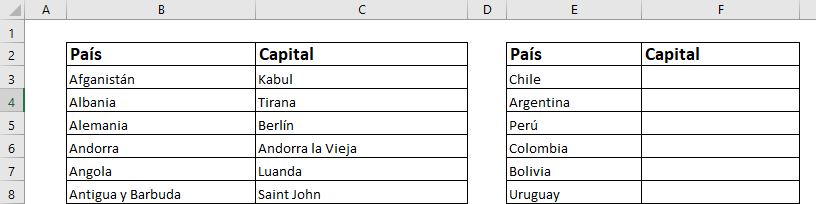
Consider the following table with countries and their capitals, and a second smaller table with a selection of countries, whose capitals do not appear.
Step 1 (with VLOOKUP): Go to the first cell of the “Capital” column in the second table, since there we want to automatically fill in the capital according to the information that appears in the first table. To achieve this, we will use the VLOOKUP function as follows:

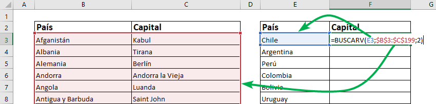
That is, we want to search for “Chile” (in blue) in the entire range of data given by the first table (in red), and when it finds it, we want it to return the value that is in the second column (in black), which contains the capital. Notice that the value of the cell that contains “Chile” is not fixed since we want this value to change as the cell changes, while the expression in red is fixed because the table where the information is searched is always the same. Then, when you drag the formula down, it will search for “Argentina” and then “Peru” and so on, but always in the same first table that we indicated with the range in red. Remember that to set rows and columns, you must put a “$” sign before the cell letter and then before the cell number.
Ninja Tip: To set cells with keyboard shortcuts, you can press the F4 key and the cell will automatically appear with the signs “$”.
Step 1 (with INDEX-MATCH): Go to the first cell of the “Capital” column in the second table, since there we want to automatically fill in the capital according to the information that appears in the first table. Now we will use the INDEX-MATCH function as follows:

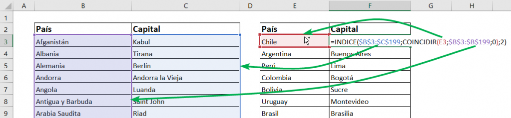
Note that, as with VLOOKUP, the range where the information should be searched is set (in blue for INDEX and then in purple for MATCH), but the cell that indicates what should be searched is left free (in red). This function performs exactly the same function as VLOOKUP in this case, so it will return exactly the same result. You may prefer to use this function if you have the information in another order (since INDEX-MATCH works in any direction), in addition to if, for example, you have the “Capital” column to the left of the “Country” column.
Ninja Tip: Since the last MATCH expression is a zero, the name match is exact.
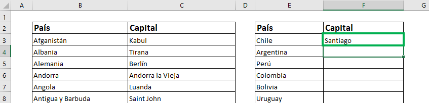
Step 2: When you finish writing the formula, press the “Enter” key. This is the result:
Step 3: Position yourself in the lower right corner of the same cell until the mouse pointer turns into a black cross, as we saw previously. Double click so that the formula is dragged to the cells below.
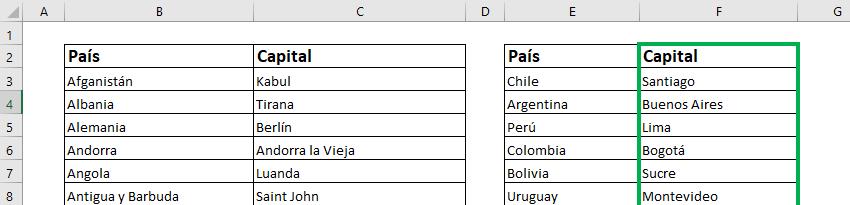
Perfect! As we saw, there are many ways to compare columns in Excel with different steps depending on what you want to achieve. Make sure you have clear objectives and you will surely be able to obtain the desired result.

Carolina Wiegand
Carolina is a doctoral student in Economics at Yale University and a Business Engineer at the Catholic University of Chile. She works with databases doing applied research on education, gender and labor market issues.