ANOVA table in Excel: how to create and interpret it

In the following article you will learn everything you need to know about an ANOVA table, its elements and its application with one and two factors.

Key information

To compare averages of different data groups we use an analysis of variance table: ANOVA (Analysis of Variance). This table contains the elements that analyze the variation of the data and helps us compare whether two or more groups are statistically different or not.

The basics of SEARCH in Excel

Purpose: The objective of an ANOVA table is to test whether two or more groups are statistically equal or different from each other.

Initial hypothesis: Also known as the “null hypothesis.” It is the initial belief that we have about the groups we have. In statistics this hypothesis is that the averages of all groups will be statistically equal.

Test F: Test made by the ANOVA table to verify whether the initial hypothesis is met, that is, whether the averages of the groups are equal or not. If the value of our “F value” is greater than a critical value, we will say that the initial hypothesis is not met, that is, the averages of the groups are statistically different.

Install the data analysis package

Before we can start analyzing an ANOVA table in Excel, we must install the data analysis package to create an ANOVA table.

Step 1: In the toolbar, click on “File” and then on “Options” (in the lower left corner).

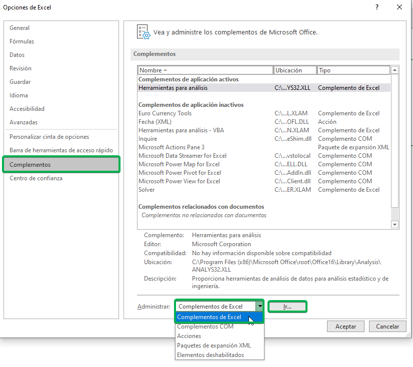
Step 2: In the new options window, we must select “Plugins”. In the “Manage” section, we select “Excel Add-ins” and then click “Go”.

Step 3: A new window will appear, in which we must check “Analysis Tools” and then click “OK”.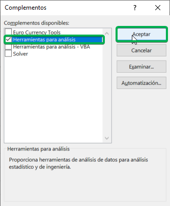

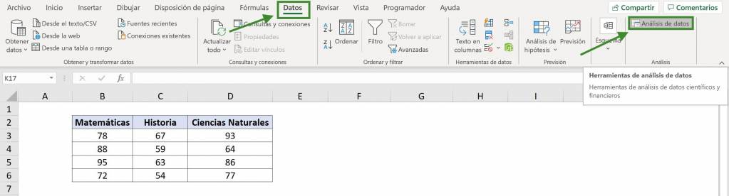
If we go to the “Data” tab on the toolbar, we will see that a new section called “Analysis” has been added, which includes the “Data Analysis” tool.

Ninja Tip: To install this package on Mac we must go to the toolbar, click on “Tools” and then on “Excel Add-ins”. Then, a new window will appear, in which we must check “Analysis Tools” and then click “OK”. With this plugin you can do linear regressions, obtain correlation coefficients, do t tests and use many other data analysis tools.

One-way ANOVA

To understand what a one-factor ANOVA table is, we will see an applied example. In this case, we have a student's grades for three different subjects: Mathematics, History and Natural Sciences.

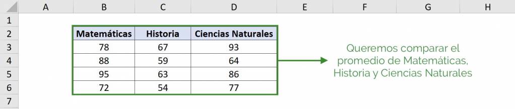
Our objective is to know if the average you have in each subject is statistically equal to the other subjects. That is, see if the average in Mathematics is the same as the average in History and Natural Sciences.

For this we must:

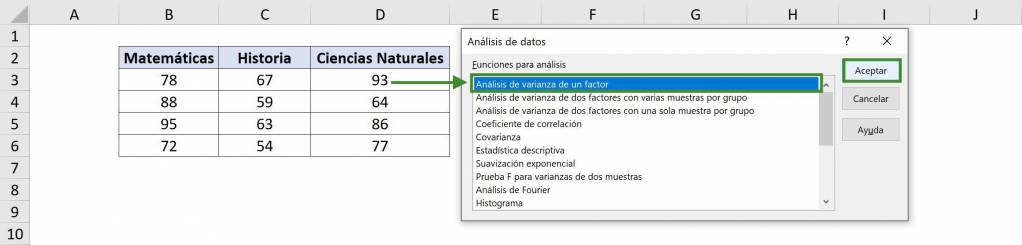
We go to the “Data” tab and click on “Data Analysis”.
In the window that opens we must select “Variance Analysis of a factor”.
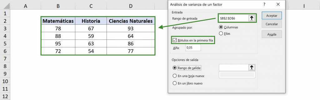
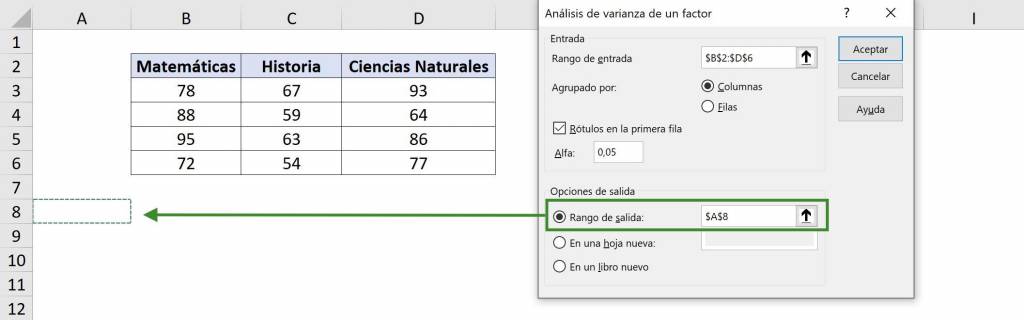
In “Input range” we select our table with data. In this case it is $B$2:$D$6 and since we include the titles we must select the option “Labels in the first row”.
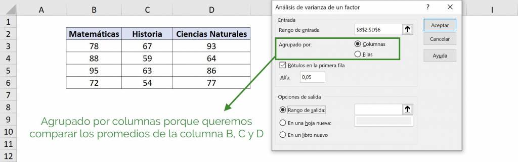
In the “Grouped by” section, we must choose the meaning of each group: since each group is a different column, we select “Columns”. This is because we want to compare one column with another.
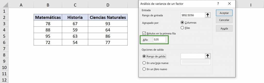
For the “Alpha” value in general 5% is used, which means that it is estimated with a confidence of 95%. If we wanted to be more strict we can choose a lower value, such as 1% (to have a reliable 99%). You can delve deeper into this concept in this article.
In “Output range” we must choose the cell where the variance analysis information will begin, that is, the upper left corner. In this case we will select $A$8. Finally we click on “Accept”.

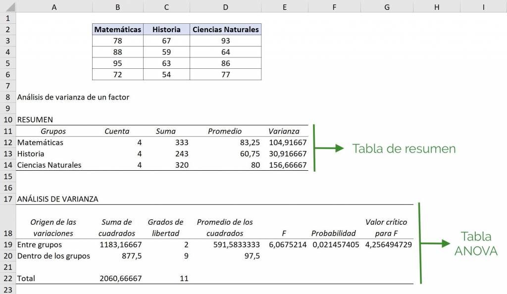
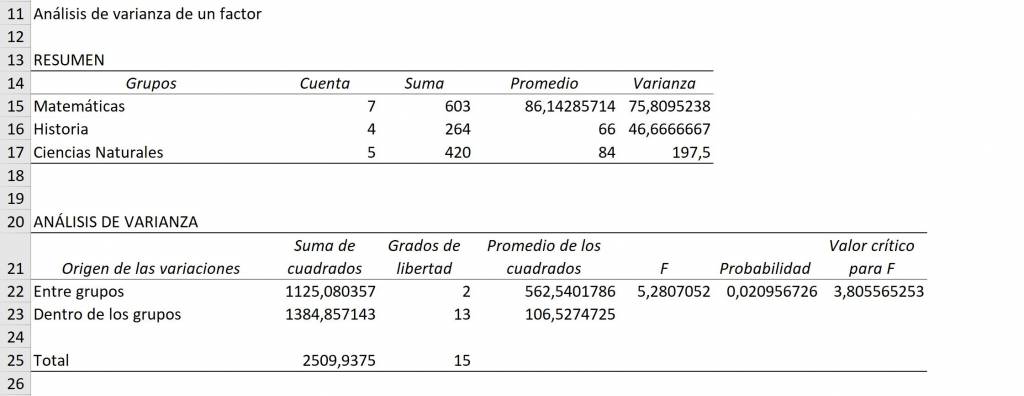
Thus, we obtain as a result a summary table of observations, average and variance of each group and an ANOVA table.

Ninja Tip: As we can see, the results are part of the spreadsheet and will be overwritten over what was previously there. This is why it is important that we worry about having enough space on the spreadsheet so as not to lose data.

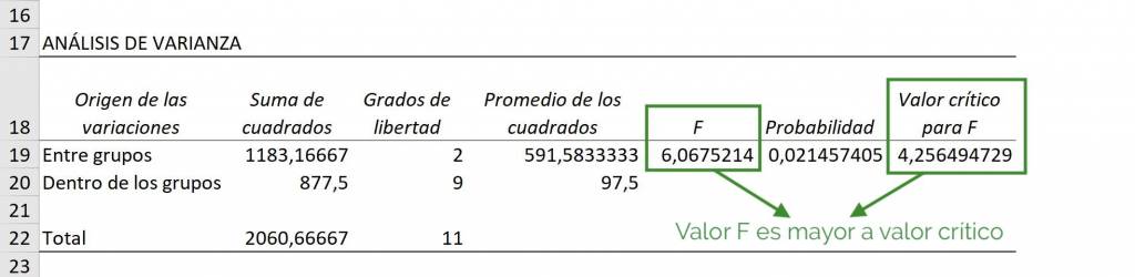
Now, when analyzing the ANOVA table our objective is to see if our initial hypothesis is met: if the F value is greater than the critical value of F, we are going to reject the hypothesis that the averages of the groups are equal. That is, if F is greater than the critical value, we are going to say at least one of the averages of these groups is statistically different.

To see this in the ANOVA table itself we go to the row that says “Between groups” and see that the F value is 6.06, while the critical F value is 4.25. As this means that the averages in Mathematics, History and Natural Sciences are not all equal to each other, that is, at least one average is different.

Ninja Tip: The critical value for F will decrease as we have more data from each group. This means that the more data we have, the more certain we can be of a statistical difference.

However, an ANOVA type analysis does not tell us which group (or groups) is (are) the different one(s) or if it is greater or less than the rest. For this we must do a t-test to see each pair of groups if they are the same or different from each other.

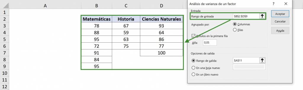
Ninja Tip: We do not need to have the same amount of data for each group to compare averages with an ANOVA table. For example, in this case we select $B$2:$D$9, leaving those cells that do not have data blank.

Obtaining the following result:

Two-way ANOVA with one sample per group

A two-factor ANOVA table consists of two types of groups and we want to study if there are differences between groups for both types. This is better understood with an example: let's think about a course that has several students and several tests have been taken.

In this case we want to see if the averages of the students are statistically equal to each other, and in addition, we want to see if the averages of the tests are statistically equal to each other. This is why it is a two-factor ANOVA: we want to study the averages of the students and the tests.

In this way we follow steps similar to those for a one-way ANOVA table:

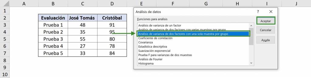
We go to the “Data” tab and click on “Data Analysis”.
In the window that opens we must select “Variance Analysis of two factors with one sample per group”.
In “Input range” we select our table with data. In this case it is $B$2:$D$7 and since we include the titles we must select the “Labels” option.
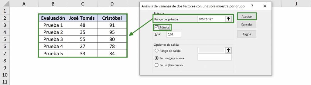
For the “Alpha” value in general 5% is used, which means that it is estimated with a confidence of 95%.
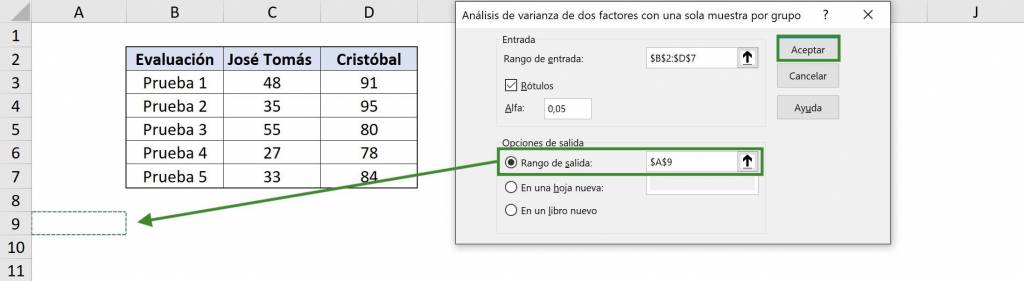
In “Output range” we must choose the cell where the variance analysis information will begin, that is, the upper left corner. In this case we will select $A$9. Finally we click on “Accept”.

Thus, we obtain as a result a summary table of observations, average and variance of each group of each type, that is, for each test for each student.

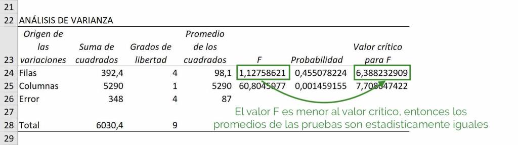
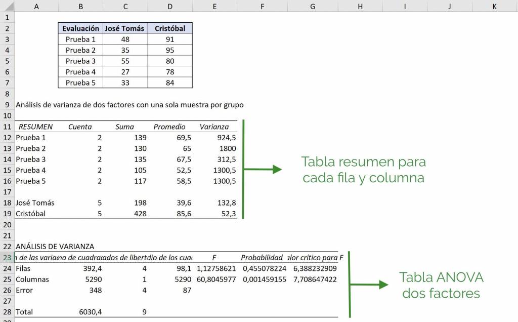Now, when analyzing the two-factor ANOVA table we have two aspects that we want to study: the difference in averages between tests and between students. When viewing the “Rows” section it is being tested between rows, that is, you are comparing whether the tests have the same averages or not. As we see, the F value is 1.12, it is less than the critical value of F (6.38). We see that the initial hypothesis is accepted in which the averages of the tests are statistically the same.

Then, for the “Columns” section, they are comparing between columns, that is, you are comparing the averages of José Tomás and Cristóbal. In the ANOVA table we see that the F value is 60.80, which is much higher than the critical value for F, which is 7.70. In this way we reject that they have the same average statistically.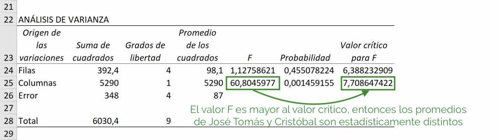

Two-way ANOVA with multiple samples per group

A two-factor ANOVA table with several samples per group, like the previous case, consists of two types of groups and we want to study if there are differences between groups for both types. However, in this case we have several data for each group. Let's look at an example: let's think that we have two schools and two subjects and that for each subject within a school we have several grades.

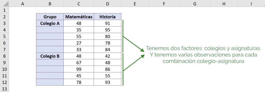
In this case we want to see if the averages of each school are statistically equal to each other, and in addition, we want to see if the averages of the subjects are statistically equal to each other. This is why it is a two-factor ANOVA: we want to study the averages of each school and each subject. Finally, since there are several samples by groups, we can study whether the “school-subject” interactions are equal between them.

In this way we follow steps similar to those for a one-factor ANOVA table in Excel:

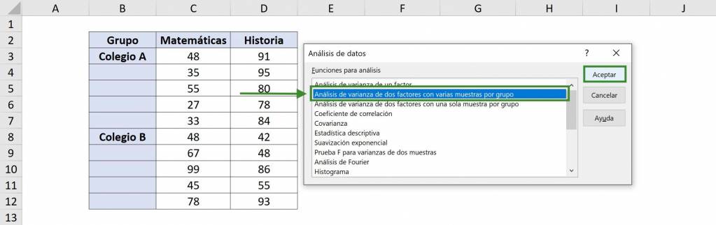
We go to the “Data” tab and click on “Data Analysis”.
In the window that opens we must select “Two-factor Variance Analysis with several samples per group”.
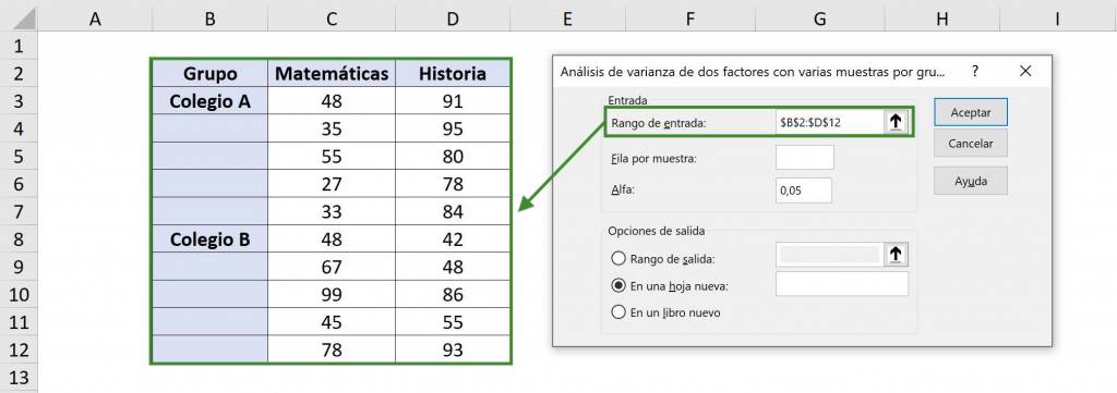
In “Input range” we select our table with data. In this case it is $B$2:$D$12, including the table titles.
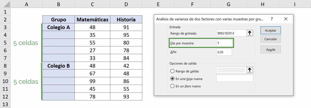
In “Row per sample” we must put how many observations we have for each group. In this case, we have 5 grades for each school, given a subject.
For the “Alpha” value in general 5% is used, which means that it is estimated with a confidence of 95%.
In “Output range” we must choose the cell where the variance analysis information will begin, that is, the upper left corner. In this case we will select $F$12. Finally we click on “Accept”.

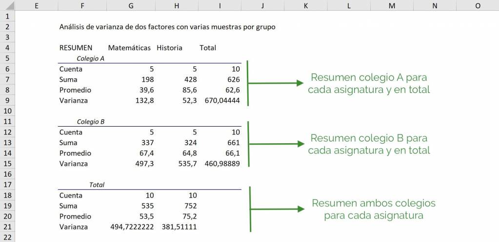
Finally, we obtain:

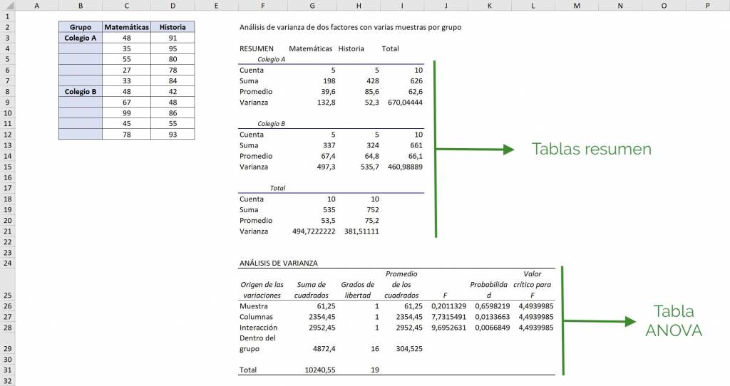Thus, we obtain a summary table for School A, for School B and for both as a set, doing an analysis for each subject.

Then, in the ANOVA table we see that in the “Sample” section columns are compared to each other, so it compares Mathematics and History and we see that we did not reject the initial hypothesis (0.20<4.49), so the averages are statistically equal. Regarding the “Columns” section, compare the average for School A with School B and we see that there is a difference between schools (7.73>4.49).

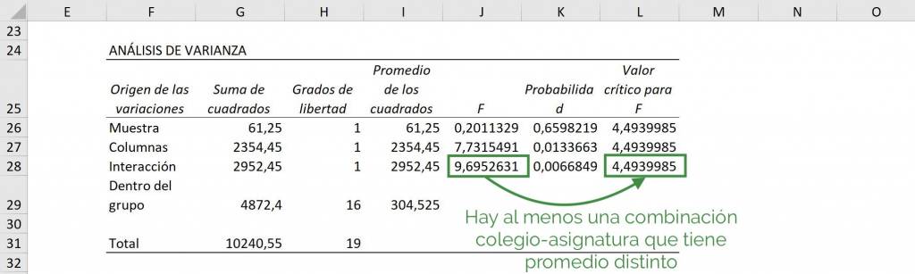
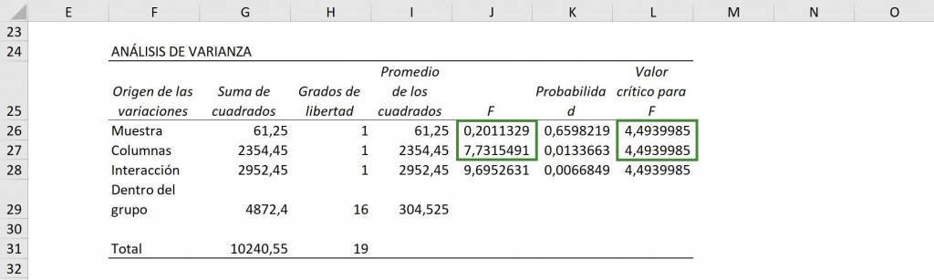Finally, we see the interaction: is School A in Mathematics, School A in History, School B in Mathematics and School B in History the same? Seeing that the value of F (9.69) is greater than the critical value of F (9.69>4.49), we see that there is at least one group that is different.